description: an algorithm used in machine learning to adjust the weights of artificial neural networks
62 results
Why Machines Learn: The Elegant Math Behind Modern AI
by
Anil Ananthaswamy
Published 15 Jul 2024
Widrow replies, “Well, this happens to spell ‘Adaptive Linear Neuron.’ And that’s it.” The line connecting ADALINE to modern neural networks (which have multiple layers and are trained using an algorithm called backpropagation) is clear. “The LMS algorithm is the foundation of backprop. And backprop is the foundation of AI,” Widrow told me. “In other words, if you trace it back, this whole field of AI right now, [it] all starts with ADALINE.” In terms of the backpropagation algorithm, this is a fair assessment. Of course, Rosenblatt’s perceptron algorithm can make similar claims. Together, Rosenblatt and Widrow laid some of the foundation stones for modern-day deep neural networks.
…
Many others hadn’t. In the 1970s, researchers were beginning to probe how to train multi-layer perceptrons (or multi-layer neural networks). The outline of an algorithm that would soon be called backpropagation, or backprop, was taking shape. But the computing power in those days wasn’t up to the task. “Nobody could do backprop on any interesting problem in [the 1970s]. You couldn’t possibly develop backprop empirically,” Hopfield said. This was the state of affairs when Hopfield entered the field, as he tried to answer his own question: “What next?” He started with an artificial neuron that was part Rosenblatt’s perceptron and part the McCulloch-Pitts neuron.
…
Hinton, and Ronald J. Williams published a pathbreaking paper on an algorithm called backpropagation. (The idea itself predated their work, but their paper put it firmly on the map.) The algorithm, which showed how to train multi-layer perceptrons, relies on calculus and optimization theory. It’d take fifteen more years before computers became powerful enough to handle the computational demands of artificial neural networks, but the “backprop” paper set a slow-burning revolution in motion. The precursor to the backpropagation algorithm, with its emphasis on calculus, however, was taking shape at about the same time as Rosenblatt was showing off his perceptron.
The Deep Learning Revolution (The MIT Press)
by
Terrence J. Sejnowski
Published 27 Sep 2018
At the same time that Geoffrey Hinton and I were working on the Boltzmann machine, David Rumelhart had developed another learning algorithm for multilayer networks that proved to be even more productive.2 Optimization Optimization is a key mathematical concept in machine learning: for many problems, a cost function can be found for which the solution is the state Backpropagating Errors 111 Box 8.1 Error Backpropagation Inputs to the backprop network are propagated feedforward: In the diagram above, the inputs on the left propagate forward through the connections (arrows) to the hidden layer of units, which in turn project to the output layer. The output is compared with the value given by a trainer, and the difference is used to update the weights to the output unit to reduce the error. The weights between the input units and the hidden layer are then updated based on backpropagating the error according to how much each weight contributes to the error.
…
See also Neural networks Associative learning, 247 ATMs (automated teller machines), 22 Attractor states, 93, 94, 94f, 95b Auditory perception and language acquisition, 184 Automated teller machines (ATMs), 22 Autonomous vehicles. See Self-driving cars Avoid being hit, 148 Backgammon, 34, 144f, 148. See also TD-Gammon backgammon board, 144f learning how to play, 143–146, 148–149 Backpropagation (backprop) learning algorithm, 114f, 217, 299n2 Backpropagation of errors (backprop), 111b, 112, 118, 148 Bag-of-words model, 251 Ballard, Dana H., 96, 297nn11–12, 314n8 Baltimore, David A., 307n5 Bar-Joseph, Ziv, 319n13 Barlow, Horace, 84, 296n8 Barry, Susan R., 294n5 Bartlett, Marian “Marni” Stewart, 181–182, 181f, 184, 308nn19–20 Barto, Andrew, 144, 146f Bartol, Thomas M., Jr., 296n14, 300n18 Basal ganglia, motivation and, 151, 153–154 Bates, Elizabeth A., 107, 298n24 Bats, 263–264 Index Bavelier, Daphne, 189–190, 309n33 Baxter (robot), 177f, 178 Bayes, Thomas, 128 Bayes networks, 128 Bear off pieces, 148 Beck, Andrew H., 287n17 Beer Bottle Pass, 4, 5f Bees, learning in, 151 Behaviorism and behaviorists, 149, 247–248 cognitive science and, 248, 249f, 250, 253 Behrens, M.
…
Rumelhart discovered how to calculate the gradient for each weight in the network by a process called the “backpropagation of errors,” or “backprop” for short (box 8.1). Starting on the output layer, where the error is known, it is easy to calculate the gradient on the input weights to the output units. The next step is to use the output layer gradients to calculate the gradients on the previous layer of weights, and so on, layer by layer, all the way back to the input layer. This is a highly efficient way to compute error gradients. Although it has neither the elegance nor the deep roots in physics that the Boltzmann machine learning algorithm has, backprop is more efficient, and it has made possible much more rapid progress.
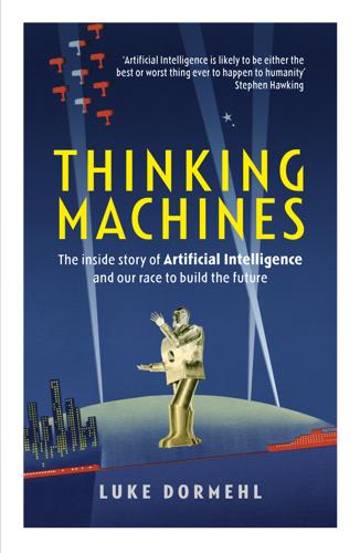
Thinking Machines: The Inside Story of Artificial Intelligence and Our Race to Build the Future
by
Luke Dormehl
Published 10 Aug 2016
For the next several years, he was responsible for a slew of groundbreaking advances in neural networks, which continue to reverberate in AI labs around the world today. Perhaps the most significant of these was helping another researcher, David Rumelhart, rediscover the ‘back-propagation’ procedure, arguably the most important algorithm in neural networks, and then producing the first convincing demonstration that back-propagation allowed neural networks to create their own internal representations. ‘Backprop’ allows a neural network to adjust its hidden layers in the event that the output it comes up with does not match the one its creator is hoping for. When this happens, the network creates an ‘error signal’ which is passed backwards through the network to the input nodes.
…
As the error is passed from layer to layer, the network’s weights are changed so that the error is minimised. Imagine, for example, that a neural net is trained to recognise images. If it analyses a picture of a dog, but mistakenly concludes that it is looking at a picture of a cat, backprop lets it go back through the previous layers of the network, with each layer modifying the weights on its incoming connections slightly so that the next time around it gets the answer correct. A classic illustration of backprop in action was a project called NETtalk, an impressive demo created in the 1980s. Co-creator Terry Sejnowski describes NETtalk as a ‘summer project’ designed to see whether a computer could learn to read aloud from written text.
…
The final piece of training data was a book featuring a transcription of children talking, along with a list of the actual phonemes spoken by the child, written down by a linguist. This meant that Sejnowski and Rosenberg were able to use the first transcript for the input layer and the second phoneme transcript for the output. By using backprop, NETtalk was able to learn exactly how to speak like a real kid. A recording of NETtalk in action shows the rapid progress the system made. At the start of training, it can only distinguish between vowels and consonants. The noise it produces sounds like vocal exercises a singer might perform to warm up his or her voice.
The Master Algorithm: How the Quest for the Ultimate Learning Machine Will Remake Our World
by
Pedro Domingos
Published 21 Sep 2015
As the network sees more and more images of your grandmother and other people, the weights gradually converge to values that let it discriminate between the two. Backpropagation, as this algorithm is known, is phenomenally more powerful than the perceptron algorithm. A single neuron could only learn straight lines. Given enough hidden neurons, a multilayer perceptron, as it’s called, can represent arbitrarily convoluted frontiers. This makes backpropagation—or simply backprop—the connectionists’ master algorithm. Backprop is an instance of a strategy that is very common in both nature and technology: if you’re in a hurry to get to the top of the mountain, climb the steepest slope you can find.
…
Neurocomputing,* edited by James Anderson and Edward Rosenfeld (MIT Press, 1988), collates many of the classic connectionist papers, including: McCulloch and Pitts on the first models of neurons; Hebb on Hebb’s rule; Rosenblatt on perceptrons; Hopfield on Hopfield networks; Ackley, Hinton, and Sejnowski on Boltzmann machines; Sejnowski and Rosenberg on NETtalk; and Rumelhart, Hinton, and Williams on backpropagation. “Efficient backprop,”* by Yann LeCun, Léon Bottou, Genevieve Orr, and Klaus-Robert Müller, in Neural Networks: Tricks of the Trade, edited by Genevieve Orr and Klaus-Robert Müller (Springer, 1998), explains some of the main tricks needed to make backprop work. Neural Networks in Finance and Investing,* edited by Robert Trippi and Efraim Turban (McGraw-Hill, 1992), is a collection of articles on financial applications of neural networks.
…
This is difficult because there is no simple linear relationship between these quantities. Rather, the cell maintains its stability through interlocking feedback loops, leading to very complex behavior. Backpropagation is well suited to this problem because of its ability to efficiently learn nonlinear functions. If we had a complete map of the cell’s metabolic pathways and enough observations of all the relevant variables, backprop could in principle learn a detailed model of the cell, with a multilayer perceptron to predict each variable as a function of its immediate causes. For the foreseeable future, however, we’ll have only partial knowledge of cells’ metabolic networks and be able to observe only a fraction of the variables we’d like to.
The Road to Conscious Machines
by
Michael Wooldridge
Published 2 Nov 2018
And PDP provided a solution to this problem in the form of an algorithm called backpropagation, more commonly referred to as backprop – probably the single most important technique in the field of neural nets. As is often the case in science, backprop seems to have been invented and reinvented a number of times over the years, but it was the specific approach introduced by the PDP researchers that definitively established it.5 Unfortunately, a proper explanation of backprop would require university-level calculus, and is far beyond the scope of this book. But the basic idea is simple enough. Backprop works by looking at cases where a neural net has made an error in its classification: this error manifests itself at the output layer of the network.
…
Artificial General Intelligence (AGI) The ambitious goal of building AI systems that have the full range of intellectual abilities that humans have: the ability to plan, reason, engage in natural language conversation, make jokes, tell stories, understand stories, play games – everything. Asilomar principles A set of principles for ethical AI developed by AI scientists and commentators in two meetings held in Asilomar, California, in 2015 and 2017. axon The component part of a neuron which connects it with other neurons. See also synapse. backprop/backpropagation The most important algorithm for training neural nets. backward chaining In knowledge-based systems, the idea that we start with a goal that we are trying to establish (e.g., ‘animal is carnivore’) and try to establish it by seeing if the goal is justified using the data we have (e.g., ‘animal eats meat’).
…
A A* 77 À la recherche du temps perdu (Proust) 205–8 accountability 257 Advanced Research Projects Agency (ARPA) 87–8 adversarial machine learning 190 AF (Artificial Flight) parable 127–9, 243 agent-based AI 136–49 agent-based interfaces 147, 149 ‘Agents That Reduce Work and Information Overload’ (Maes) 147–8 AGI (Artificial General Intelligence) 41 AI – difficulty of 24–8 – ethical 246–62, 284, 285 – future of 7–8 – General 42, 53, 116, 119–20 – Golden Age of 47–88 – history of 5–7 – meaning of 2–4 – narrow 42 – origin of name 51–2 – strong 36–8, 41, 309–14 – symbolic 42–3, 44 – varieties of 36–8 – weak 36–8 AI winter 87–8 AI-complete problems 84 ‘Alchemy and AI’ (Dreyfus) 85 AlexNet 187 algorithmic bias 287–9, 292–3 alienation 274–7 allocative harm 287–8 AlphaFold 214 AlphaGo 196–9 AlphaGo Zero 199 AlphaZero 199–200 Alvey programme 100 Amazon 275–6 Apple Watch 218 Argo AI 232 arithmetic 24–6 Arkin, Ron 284 ARPA (Advanced Research Projects Agency) 87–8 Artificial Flight (AF) parable 127–9, 243 Artificial General Intelligence (AGI) 41 artificial intelligence see AI artificial languages 56 Asilomar principles 254–6 Asimov, Isaac 244–6 Atari 2600 games console 192–6, 327–8 augmented reality 296–7 automated diagnosis 220–1 automated translation 204–8 automation 265, 267–72 autonomous drones 282–4 Autonomous Vehicle Disengagement Reports 231 autonomous vehicles see driverless cars autonomous weapons 281–7 autonomy levels 227–8 Autopilot 228–9 B backprop/backpropagation 182–3 backward chaining 94 Bayes nets 158 Bayes’ Theorem 155–8, 365–7 Bayesian networks 158 behavioural AI 132–7 beliefs 108–10 bias 172 black holes 213–14 Blade Runner 38 Blocks World 57–63, 126–7 blood diseases 94–8 board games 26, 75–6 Boole, George 107 brains 43, 306, 330–1 see also electronic brains branching factors 73 Breakout (video game) 193–5 Brooks, Rodney 125–9, 132, 134, 243 bugs 258 C Campaign to Stop Killer Robots 286 CaptionBot 201–4 Cardiogram 215 cars 27–8, 155, 223–35 certainty factors 97 ceteris paribus preferences 262 chain reactions 242–3 chatbots 36 checkers 75–7 chess 163–4, 199 Chinese room 311–14 choice under uncertainty 152–3 combinatorial explosion 74, 80–1 common values and norms 260 common-sense reasoning 121–3 see also reasoning COMPAS 280 complexity barrier 77–85 comprehension 38–41 computational complexity 77–85 computational effort 129 computers – decision making 23–4 – early developments 20 – as electronic brains 20–4 – intelligence 21–2 – programming 21–2 – reliability 23 – speed of 23 – tasks for 24–8 – unsolved problems 28 ‘Computing Machinery and Intelligence’ (Turing) 32 confirmation bias 295 conscious machines 327–30 consciousness 305–10, 314–17, 331–4 consensus reality 296–8 consequentialist theories 249 contradictions 122–3 conventional warfare 286 credit assignment problem 173, 196 Criado Perez, Caroline 291–2 crime 277–81 Cruise Automation 232 curse of dimensionality 172 cutlery 261 Cybernetics (Wiener) 29 Cyc 114–21, 208 D DARPA (Defense Advanced Research Projects Agency) 87–8, 225–6 Dartmouth summer school 1955 50–2 decidable problems 78–9 decision problems 15–19 deduction 106 deep learning 168, 184–90, 208 DeepBlue 163–4 DeepFakes 297–8 DeepMind 167–8, 190–200, 220–1, 327–8 Defense Advanced Research Projects Agency (DARPA) 87–8, 225–6 dementia 219 DENDRAL 98 Dennett, Daniel 319–25 depth-first search 74–5 design stance 320–1 desktop computers 145 diagnosis 220–1 disengagements 231 diversity 290–3 ‘divide and conquer’ assumption 53–6, 128 Do-Much-More 35–6 dot-com bubble 148–9 Dreyfus, Hubert 85–6, 311 driverless cars 27–8, 155, 223–35 drones 282–4 Dunbar, Robin 317–19 Dunbar’s number 318 E ECAI (European Conference on AI) 209–10 electronic brains 20–4 see also computers ELIZA 32–4, 36, 63 employment 264–77 ENIAC 20 Entscheidungsproblem 15–19 epiphenomenalism 316 error correction procedures 180 ethical AI 246–62, 284, 285 European Conference on AI (ECAI) 209–10 evolutionary development 331–3 evolutionary theory 316 exclusive OR (XOR) 180 expected utility 153 expert systems 89–94, 123 see also Cyc; DENDRAL; MYCIN; R1/XCON eye scans 220–1 F Facebook 237 facial recognition 27 fake AI 298–301 fake news 293–8 fake pictures of people 214 Fantasia 261 feature extraction 171–2 feedback 172–3 Ferranti Mark 1 20 Fifth Generation Computer Systems Project 113–14 first-order logic 107 Ford 232 forward chaining 94 Frey, Carl 268–70 ‘The Future of Employment’ (Frey & Osborne) 268–70 G game theory 161–2 game-playing 26 Gangs Matrix 280 gender stereotypes 292–3 General AI 41, 53, 116, 119–20 General Motors 232 Genghis robot 134–6 gig economy 275 globalization 267 Go 73–4, 196–9 Golden Age of AI 47–88 Google 167, 231, 256–7 Google Glass 296–7 Google Translate 205–8, 292–3 GPUs (Graphics Processing Units) 187–8 gradient descent 183 Grand Challenges 2004/5 225–6 graphical user interfaces (GUI) 144–5 Graphics Processing Units (GPUs) 187–8 GUI (graphical user interfaces) 144–5 H hard problem of consciousness 314–17 hard problems 84, 86–7 Harm Assessment Risk Tool (HART) 277–80 Hawking, Stephen 238 healthcare 215–23 Herschel, John 304–6 Herzberg, Elaine 230 heuristic search 75–7, 164 heuristics 91 higher-order intentional reasoning 323–4, 328 high-level programming languages 144 Hilbert, David 15–16 Hinton, Geoff 185–6, 221 HOMER 141–3, 146 homunculus problem 315 human brain 43, 306, 330–1 human intuition 311 human judgement 222 human rights 277–81 human-level intelligence 28–36, 241–3 ‘humans are special’ argument 310–11 I image classification 186–7 image-captioning 200–4 ImageNet 186–7 Imitation Game 30 In Search of Lost Time (Proust) 205–8 incentives 261 indistinguishability 30–1, 37, 38 Industrial Revolutions 265–7 inference engines 92–4 insurance 219–20 intelligence 21–2, 127–8, 200 – human-level 28–36, 241–3 ‘Intelligence Without Representation’ (Brooks) 129 Intelligent Knowledge-Based Systems 100 intentional reasoning 323–4, 328 intentional stance 321–7 intentional systems 321–2 internal mental phenomena 306–7 Internet chatbots 36 intuition 311 inverse reinforcement learning 262 Invisible Women (Criado Perez) 291–2 J Japan 113–14 judgement 222 K Kasparov, Garry 163 knowledge bases 92–4 knowledge elicitation problem 123 knowledge graph 120–1 Knowledge Navigator 146–7 knowledge representation 91, 104, 129–30, 208 knowledge-based AI 89–123, 208 Kurzweil, Ray 239–40 L Lee Sedol 197–8 leisure 272 Lenat, Doug 114–21 lethal autonomous weapons 281–7 Lighthill Report 87–8 LISP 49, 99 Loebner Prize Competition 34–6 logic 104–7, 121–2 logic programming 111–14 logic-based AI 107–11, 130–2 M Mac computers 144–6 McCarthy, John 49–52, 107–8, 326–7 machine learning (ML) 27, 54–5, 168–74, 209–10, 287–9 machines with mental states 326–7 Macintosh computers 144–6 magnetic resonance imaging (MRI) 306 male-orientation 290–3 Manchester Baby computer 20, 24–6, 143–4 Manhattan Project 51 Marx, Karl 274–6 maximizing expected utility 154 Mercedes 231 Mickey Mouse 261 microprocessors 267–8, 271–2 military drones 282–4 mind modelling 42 mind-body problem 314–17 see also consciousness minimax search 76 mining industry 234 Minsky, Marvin 34, 52, 180 ML (machine learning) 27, 54–5, 168–74, 209–10, 287–9 Montezuma’s Revenge (video game) 195–6 Moore’s law 240 Moorfields Eye Hospital 220–1 moral agency 257–8 Moral Machines 251–3 MRI (magnetic resonance imaging) 306 multi-agent systems 160–2 multi-layer perceptrons 177, 180, 182 Musk, Elon 238 MYCIN 94–8, 217 N Nagel, Thomas 307–10 narrow AI 42 Nash, John Forbes Jr 50–1, 161 Nash equilibrium 161–2 natural languages 56 negative feedback 173 neural nets/neural networks 44, 168, 173–90, 369–72 neurons 174 Newell, Alan 52–3 norms 260 NP-complete problems 81–5, 164–5 nuclear energy 242–3 nuclear fusion 305 O ontological engineering 117 Osborne, Michael 268–70 P P vs NP problem 83 paperclips 261 Papert, Seymour 180 Parallel Distributed Processing (PDP) 182–4 Pepper 299 perception 54 perceptron models 174–81, 183 Perceptrons (Minsky & Papert) 180–1, 210 personal healthcare management 217–20 perverse instantiation 260–1 Phaedrus 315 physical stance 319–20 Plato 315 police 277–80 Pratt, Vaughan 117–19 preference relations 151 preferences 150–2, 154 privacy 219 problem solving and planning 55–6, 66–77, 128 programming 21–2 programming languages 144 PROLOG 112–14, 363–4 PROMETHEUS 224–5 protein folding 214 Proust, Marcel 205–8 Q qualia 306–7 QuickSort 26 R R1/XCON 98–9 radiology 215, 221 railway networks 259 RAND Corporation 51 rational decision making 150–5 reasoning 55–6, 121–3, 128–30, 137, 315–16, 323–4, 328 regulation of AI 243 reinforcement learning 172–3, 193, 195, 262 representation harm 288 responsibility 257–8 rewards 172–3, 196 robots – as autonomous weapons 284–5 – Baye’s theorem 157 – beliefs 108–10 – fake 299–300 – indistinguishability 38 – intentional stance 326–7 – SHAKEY 63–6 – Sophia 299–300 – Three Laws of Robotics 244–6 – trivial tasks 61 – vacuum cleaning 132–6 Rosenblatt, Frank 174–81 rules 91–2, 104, 359–62 Russia 261 Rutherford, Ernest (1st Baron Rutherford of Nelson) 242 S Sally-Anne tests 328–9, 330 Samuel, Arthur 75–7 SAT solvers 164–5 Saudi Arabia 299–300 scripts 100–2 search 26, 68–77, 164, 199 search trees 70–1 Searle, John 311–14 self-awareness 41, 305 see also consciousness semantic nets 102 sensors 54 SHAKEY the robot 63–6 SHRDLU 56–63 Simon, Herb 52–3, 86 the Singularity 239–43 The Singularity is Near (Kurzweil) 239 Siri 149, 298 Smith, Matt 201–4 smoking 173 social brain 317–19 see also brains social media 293–6 social reasoning 323, 324–5 social welfare 249 software agents 143–9 software bugs 258 Sophia 299–300 sorting 26 spoken word translation 27 STANLEY 226 STRIPS 65 strong AI 36–8, 41, 309–14 subsumption architecture 132–6 subsumption hierarchy 134 sun 304 supervised learning 169 syllogisms 105, 106 symbolic AI 42–3, 44, 181 synapses 174 Szilard, Leo 242 T tablet computers 146 team-building problem 78–81, 83 Terminator narrative of AI 237–9 Tesla 228–9 text recognition 169–71 Theory of Mind (ToM) 330 Three Laws of Robotics 244–6 TIMIT 292 ToM (Theory of Mind) 330 ToMnet 330 TouringMachines 139–41 Towers of Hanoi 67–72 training data 169–72, 288–9, 292 translation 204–8 transparency 258 travelling salesman problem 82–3 Trolley Problem 246–53 Trump, Donald 294 Turing, Alan 14–15, 17–19, 20, 24–6, 77–8 Turing Machines 18–19, 21 Turing test 29–38 U Uber 168, 230 uncertainty 97–8, 155–8 undecidable problems 19, 78 understanding 201–4, 312–14 unemployment 264–77 unintended consequences 263 universal basic income 272–3 Universal Turing Machines 18, 19 Upanishads 315 Urban Challenge 2007 226–7 utilitarianism 249 utilities 151–4 utopians 271 V vacuum cleaning robots 132–6 values and norms 260 video games 192–6, 327–8 virtue ethics 250 Von Neumann and Morgenstern model 150–5 Von Neumann architecture 20 W warfare 285–6 WARPLAN 113 Waymo 231, 232–3 weak AI 36–8 weapons 281–7 wearable technology 217–20 web search 148–9 Weizenbaum, Joseph 32–4 Winograd schemas 39–40 working memory 92 X XOR (exclusive OR) 180 Z Z3 computer 19–20 PELICAN BOOKS Economics: The User’s Guide Ha-Joon Chang Human Evolution Robin Dunbar Revolutionary Russia: 1891–1991 Orlando Figes The Domesticated Brain Bruce Hood Greek and Roman Political Ideas Melissa Lane Classical Literature Richard Jenkyns Who Governs Britain?
Genius Makers: The Mavericks Who Brought A. I. To Google, Facebook, and the World
by
Cade Metz
Published 15 Mar 2021
The morning of his wedding, he disappeared for half an hour to mail a package to the editors of Nature, one of the world’s leading science journals. The package contained a research paper describing backpropagation, written with Rumelhart and a Northeastern University professor named Ronald Williams. It was published later that year. This was the kind of academic moment that goes unnoticed across the larger world, but in the wake of the paper, neural networks entered a new age of optimism and, indeed, progress, riding a larger wave of AI funding as the field emerged from its first long winter. “Backprop,” as researchers called it, was not just an idea. One of the first practical applications came in 1987.
…
Hinton liked to say that “old ideas are new”—that scientists should never give up on an idea unless someone had proven it wouldn’t work. Twenty years earlier, Rosenblatt had proven that backpropagation wouldn’t work, so Hinton gave up on it. Then Rumelhart made this small suggestion. Over the next several weeks, the two men got to work building a system that began with random weights, and it could break symmetry. It could assign a different weight to each neuron. And in setting these weights, the system could actually recognize patterns in images. These were simple images. The system couldn’t recognize a dog or a cat or a car, but thanks to backpropagation, it could now handle that thing called “exclusive-or,” moving beyond the flaw that Marvin Minsky pinpointed in neural networks more than a decade earlier.
…
Later, Hinton discovered he was paid about a third less than his colleagues ($26,000 versus $35,000), but he’d found a home for his unorthodox research. He continued work on the Boltzmann Machine, often driving to Baltimore on weekends so he could collaborate with Sejnowski in the lab at Johns Hopkins, and somewhere along the way, he also started tinkering with backpropagation, reckoning it would throw up useful comparisons. He thought he needed something he could compare with the Boltzmann Machine, and backpropagation was as good as anything else. An old idea was new. At Carnegie Mellon, he had more than just the opportunity to explore these two projects. He had better, faster computer hardware. This drove the research forward, allowing these mathematical systems to learn more from more data.
Deep Medicine: How Artificial Intelligence Can Make Healthcare Human Again
by
Eric Topol
Published 1 Jan 2019
One, called the “The Elephant in the Room,” literally showed the inability for deep learning to accurately recognize the image of an elephant when it was introduced to a living room scene that included a couch, a person, a chair, and books on a shelf.6 On the flip side, the vulnerability of deep neural networks was exemplified by seeing a ghost—identifying a person who was not present in the image.7 Some experts believe that deep learning has hit its limits and it’ll be hard-pressed to go beyond the current level of narrow functionality. Geoffrey Hinton, the father of deep learning, has even called the entire methodology into question.8 Although he invented backpropagation, the method for error correction in neural networks, he recently said he had become “deeply suspicious” of backprop, saying his view had become that we should “throw it all away and start again.”9 Pointing to the technology’s reliance on extensive labeling, he projected that the inefficiencies resulting from that dependence “may lead to their demise.”10 Hinton is intent on narrowing the chasm between AI and children and has introduced the concept of capsule networks.11 He’s clearly excited about the idea of bridging biology and computer science, which for him requires going beyond the flat layers of today’s deep neural networks: capsule networks have vertical columns to simulate the brain’s neocortex.
…
In particular, it will be the century of the human brain—the most complex piece of highly excitable matter in the known universe.”52 We’re also seeing how advances in computer science can help us better understand our brains, not just by sorting out the mechanics by which the brain works, but by giving us the conceptual tools to understand how it works. In Chapter 4 I reviewed backpropagation, the way neural networks learn by comparing their output with the desired output and adjusting in reverse order of execution. That critical concept wasn’t thought to be biologically plausible. Recent work has actually borne out the brain’s way of using backpropagation to implement algorithms.53 Similarly, most neuroscientists thought biological neural networks, as compared with artificial neural networks, only do supervised learning.
…
Geoffrey Hinton, the father of deep learning, has even called the entire methodology into question.8 Although he invented backpropagation, the method for error correction in neural networks, he recently said he had become “deeply suspicious” of backprop, saying his view had become that we should “throw it all away and start again.”9 Pointing to the technology’s reliance on extensive labeling, he projected that the inefficiencies resulting from that dependence “may lead to their demise.”10 Hinton is intent on narrowing the chasm between AI and children and has introduced the concept of capsule networks.11 He’s clearly excited about the idea of bridging biology and computer science, which for him requires going beyond the flat layers of today’s deep neural networks: capsule networks have vertical columns to simulate the brain’s neocortex. While capsule architecture has yet to improve network performance, it’s helpful to remember that backprop took decades to be accepted. It’s much too early to know whether capsule networks will follow suit, but just the fact that he has punched holes in current DNN methodology is disconcerting. The triumph of AlphaGo Zero also brings up several issues. The Nature paper was announced with much fanfare; the authors made the claim in the title “Mastering the Game of Go Without Human Knowledge.”12 When I questioned Gary Marcus on this point, he said that was “ridiculous.”
Driverless: Intelligent Cars and the Road Ahead
by
Hod Lipson
and
Melba Kurman
Published 22 Sep 2016
Compare this to Rosenblatt’s original machine that offered just two crisp outputs: either a 1 or a 0; the light bulb providing the “answer” was either on or off, with nothing in between. The second improvement that Werbos provided was a new training algorithm called error backpropagation, or backprop. Now that the artificial neurons could handle uncertainty in the form of fractional numbers, the backprop algorithm could be used to train a neural network with more than one layer. One major limitation of Rosenblatt’s Perceptron had been that its output layer could handle only two answers rather than a range; therefore, the learning curve was too steep to climb.
…
In a fate similar to that which befell the Perceptron, the Neocognitron couldn’t perform at a reasonable speed using the computing power available in the 1980s. It seemed that Werbos’s backprop training algorithm was not powerful enough to train networks more than three or four layers deep. The reinforcement signal would fizzle out and network learning would cease because it couldn’t tell which connections were responsible for wrong answers. We know today that the backprop algorithm was correct in concept, but in execution it lacked the underlying technology and data that it needed to work as its inventor intended. During the 1990s and 2000s, some researchers tried to make up for the lack of computer power and data by using “shallower” networks, with just two layers of artificial neurons.
…
But when presented with pictures depicting somewhat similar four-legged animals, the network’s performance would deteriorate to just above randomness, somewhat like a student circling just any answer to get through a multiple-choice exam. Nevertheless, hope springs eternal. Better digital-camera technology combined with the timely release of Werbos’s backprop algorithm sparked new interest in the field of neural-network research, effectively ending the long AI winter of the 1960s and 1970s. If you dig through research papers from the late 1980s and 1990s, you’ll find the relics of this brief period of euphoria. Researchers attempted to apply neural networks to classify everything under the sun: images, text, and sound.
Architects of Intelligence
by
Martin Ford
Published 16 Nov 2018
Opening the hood and delving into the details of these terms is entirely optional: BACKPROPAGATION (or BACKPROP) is the learning algorithm used in deep learning systems. As a neural network is trained (see supervised learning below), information propagates back through the layers of neurons that make up the network and causes a recalibration of the settings (or weights) for the individual neurons. The result is that the entire network gradually homes in on the correct answer. Geoff Hinton co-authored the seminal academic paper on backpropagation in 1986. He explains backprop further in his interview. An even more obscure term is GRADIENT DESCENT.
…
We don’t know for sure, but there are some reasons now for believing that the brain might not use backpropagation. I said that if the brain doesn’t use backpropagation, then whatever the brain is using would be an interesting candidate for artificial systems. I didn’t at all mean that we should throw out backpropagation. Backpropagation is the mainstay of all the deep learning that works, and I don’t think we should get rid of it. MARTIN FORD: Presumably, it could be refined going forward? GEOFFREY HINTON: There’s going to be all sorts of ways of improving it, and there may well be other algorithms that are not backpropagation that also work, but I don’t think we should stop doing backpropagation.
…
In particular, something called the support vector machine did better at recognizing handwritten digits than backpropagation, and handwritten digits had been a classic example of backpropagation doing something really well. Because of that, the machine learning community really lost interest in backpropagation. They decided that there was too much fiddling involved, it didn’t work well enough to be worth all that fiddling, and it was hopeless to think that just from the inputs and outputs you could learn multiple layers of hidden representations. Each layer would be a whole bunch of feature detectors that represent in a particular way. The idea of backpropagation was that you’d learn lots of layers, and then you’d be able to do amazing things, but we had great difficulty learning more than a few layers, and we couldn’t do amazing things.
Artificial Intelligence: A Guide for Thinking Humans
by
Melanie Mitchell
Published 14 Oct 2019
And by the late 1970s and early ’80s, several of these groups had definitively rebutted Minsky and Papert’s speculations on the “sterility” of multilayer neural networks by developing a general learning algorithm—called back-propagation—for training these networks. As its name implies, back-propagation is a way to take an error observed at the output units (for example, a high confidence for the wrong digit in the example of figure 4) and to “propagate” the blame for that error backward (in figure 4, this would be from right to left) so as to assign proper blame to each of the weights in the network. This allows back-propagation to determine how much to change each weight in order to reduce the error. Learning in neural networks simply consists in gradually modifying the weights on connections so that each output’s error gets as close to 0 as possible on all training examples.
…
Learning in neural networks simply consists in gradually modifying the weights on connections so that each output’s error gets as close to 0 as possible on all training examples. While the mathematics of back-propagation is beyond the scope of my discussion here, I’ve included some details in the notes.2 Back-propagation will work (in principle at least) no matter how many inputs, hidden units, or output units your neural network has. While there is no mathematical guarantee that back-propagation will settle on the correct weights for a network, in practice it has worked very well on many tasks that are too hard for simple perceptrons. For example, I trained both a perceptron and a two-layer neural network, each with 324 inputs and 10 outputs, on the handwritten-digit-recognition task, using sixty thousand examples, and then tested how well each was able to recognize ten thousand new examples.
…
As a graduate student and postdoctoral fellow, he was fascinated by Rosenblatt’s perceptrons and Fukushima’s neocognitron, but noted that the latter lacked a good supervised-learning algorithm. Along with other researchers (most notably, his postdoctoral advisor Geoffrey Hinton), LeCun helped develop such a learning method—essentially the same form of back-propagation used on ConvNets today.1 In the 1980s and ’90s, while working at Bell Labs, LeCun turned to the problem of recognizing handwritten digits and letters. He combined ideas from the neocognitron with the back-propagation algorithm to create the semi-eponymous “LeNet”—one of the earliest ConvNets. LeNet’s handwritten-digit-recognition abilities made it a commercial success: in the 1990s and into the 2000s it was used by the U.S.
How the Mind Works
by
Steven Pinker
Published 1 Jan 1997
That signal can serve as a surrogate teaching signal which may be used to adjust the hidden layer’s inputs. The connections from the input layer to each hidden unit can be nudged up or down to reduce the hidden unit’s tendency to overshoot or undershoot, given the current input pattern. This procedure, called “error back-propagation” or simply “backprop,” can be iterated backwards to any number of layers. We have reached what many psychologists treat as the height of the neural-network modeler’s art. In a way, we have come full circle, because a hidden-layer network is like the arbitrary road map of logic gates that McCulloch and Pitts proposed as their neuro-logical computer.
…
Or are the networks more like building blocks that aren’t humanly smart until they are assembled into structured representations and programs? A school called connectionism, led by the psychologists David Rumelhart and James McClelland, argues that simple networks by themselves can account for most of human intelligence. In its extreme form, connectionism says that the mind is one big hidden-layer back-propagation network, or perhaps a battery of similar or identical ones, and intelligence emerges when a trainer, the environment, tunes the connection weights. The only reason that humans are smarter than rats is that our networks have more hidden layers between stimulus and response and we live in an environment of other humans who serve as network trainers.
…
Towards a psychology of food and eating: From motivation to module to model to marker, morality, meaning, and metaphor. Current Directions in Psychological Science, 5, 18–24. Rozin, P., & Fallon, A. 1987. A perspective on disgust. Psychological Review, 94, 23–41. Rumelhart, D. E., Hinton, G. E., & Williams, R. J. 1986. Learning representations by back-propagating errors. Nature, 323, 533–536. Rumelhart, D. E., & McClelland, J. L. 1986a. PDP models and general issues in cognitive science. In Rumelhart, McClelland, & the PDP Research Group, 1986. Rumelhart, D. E., & McClelland, J. L. 1986b. On learning the past tenses of English verbs. Implicit rules or parallel distributed processing?
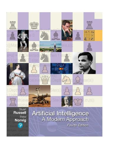
Artificial Intelligence: A Modern Approach
by
Stuart Russell
and
Peter Norvig
Published 14 Jul 2019
The policy loss curve starts at (0, 0.5), drops linearly until the point (10, 0.25). The curve then remains horizontally constant until it ends at (500, 0.25). Figure 22.6Illustration of the back-propagation of gradient information in an arbitrary computation graph. The forward computation of the output of the network proceeds from left to right, while the back-propagation of gradients proceeds from right to left. The back-propagation process passes messages back along each link in the network. At each node, the incoming messages are collected and new messages are calculated to pass back to the next layer. As the figure shows, the messages are all partial derivatives of the loss L.
…
Weight-sharing, as used in convolutional networks (Section 22.3) and recurrent networks (Section 22.6), is handled simply by treating each shared weight as a single node with multiple outgoing arcs in the computation graph. During back-propagation, this results in multiple incoming gradient messages. By Equation (22.11), this means that the gradient for the shared weight is the sum of the gradient contributions from each place it is used in the network. It is clear from this description of the back-propagation process that its computational cost is linear in the number of nodes in the computation graph, just like the cost of the forward computation. Furthermore, because the node types are typically fixed when the network is designed, all of the gradient computations can be prepared in symbolic form in advance and compiled into very efficient code for each node in the graph.
…
The two-volume “PDP” (Parallel Distributed Processing) anthology (Rumelhart and McClelland, 1986) helped to spread the gospel, so to speak, particularly in the psychology and cognitive science communities. The most important development of this period was the back-propagation algorithm for training multilayer networks. The back-propagation algorithm was discovered independently several times in different contexts (Kelley, 1960; Bryson, 1962; Dreyfus, 1962; Bryson and Ho, 1969; Werbos, 1974; Parker, 1985) and Stuart Dreyfus (1990) calls it the “Kelley–Bryson gradient procedure.” Although Werbos had applied it to neural networks, this idea did not become widely known until a paper by David Rumelhart, Geoff Hinton, and Ron Williams (1986) appeared in Nature giving a nonmathematical presentation of the algorithm.
The Elements of Statistical Learning (Springer Series in Statistics)
by
Trevor Hastie
,
Robert Tibshirani
and
Jerome Friedman
Published 25 Aug 2009
From their definitions, these errors satisfy K X T βkm δki , (11.15) smi = σ ′ (αm xi ) k=1 known as the back-propagation equations. Using this, the updates in (11.13) can be implemented with a two-pass algorithm. In the forward pass, the current weights are fixed and the predicted values fˆk (xi ) are computed from formula (11.5). In the backward pass, the errors δki are computed, and then back-propagated via (11.15) to give the errors smi . Both sets of errors are then used to compute the gradients for the updates in (11.13), via (11.14). 11.5 Some Issues in Training Neural Networks 397 This two-pass procedure is what is known as back-propagation. It has also been called the delta rule (Widrow and Hoff, 1960).
…
Instead some regularization is needed: this is achieved directly through a penalty term, or indirectly by early stopping. Details are given in the next section. The generic approach to minimizing R(θ) is by gradient descent, called back-propagation in this setting. Because of the compositional form of the model, the gradient can be easily derived using the chain rule for differentiation. This can be computed by a forward and backward sweep over the network, keeping track only of quantities local to each unit. 396 Neural Networks Here is back-propagation in detail for squared error loss. Let zmi = T xi ), from (11.5) and let zi = (z1i , z2i , . . . , zM i ). Then we have σ(α0m + αm N X R(θ) ≡ Ri i=1 K N X X = (yik − fk (xi ))2 , (11.11) i=1 k=1 with derivatives ∂Ri = −2(yik − fk (xi ))gk′ (βkT zi )zmi , ∂βkm K X ∂Ri T 2(yik − fk (xi ))gk′ (βkT zi )βkm σ ′ (αm xi )xiℓ . =− ∂αmℓ (11.12) k=1 Given these derivatives, a gradient descent update at the (r + 1)st iteration has the form (r+1) βkm (r+1) αmℓ (r) = βkm − γr = (r) αmℓ − γr N X ∂Ri (r) i=1 ∂βkm N X ∂Ri (r) i=1 ∂αmℓ where γr is the learning rate, discussed below.
…
It has also been called the delta rule (Widrow and Hoff, 1960). The computational components for cross-entropy have the same form as those for the sum of squares error function, and are derived in Exercise 11.3. The advantages of back-propagation are its simple, local nature. In the back propagation algorithm, each hidden unit passes and receives information only to and from units that share a connection. Hence it can be implemented efficiently on a parallel architecture computer. The updates in (11.13) are a kind of batch learning, with the parameter updates being a sum over all of the training cases. Learning can also be carried out online—processing each observation one at a time, updating the gradient after each training case, and cycling through the training cases many times.
Data Science from Scratch: First Principles with Python
by
Joel Grus
Published 13 Apr 2015
The result is a network that performs “or, but not and,” which is precisely XOR (Figure 18-3). Figure 18-3. A neural network for XOR Backpropagation Usually we don’t build neural networks by hand. This is in part because we use them to solve much bigger problems — an image recognition problem might involve hundreds or thousands of neurons. And it’s in part because we usually won’t be able to “reason out” what the neurons should be. Instead (as usual) we use data to train neural networks. One popular approach is an algorithm called backpropagation that has similarities to the gradient descent algorithm we looked at earlier. Imagine we have a training set that consists of input vectors and corresponding target output vectors.
…
At which point we’re ready to build our neural network: random.seed(0) # to get repeatable results input_size = 25 # each input is a vector of length 25 num_hidden = 5 # we'll have 5 neurons in the hidden layer output_size = 10 # we need 10 outputs for each input # each hidden neuron has one weight per input, plus a bias weight hidden_layer = [[random.random() for __ in range(input_size + 1)] for __ in range(num_hidden)] # each output neuron has one weight per hidden neuron, plus a bias weight output_layer = [[random.random() for __ in range(num_hidden + 1)] for __ in range(output_size)] # the network starts out with random weights network = [hidden_layer, output_layer] And we can train it using the backpropagation algorithm: # 10,000 iterations seems enough to converge for __ in range(10000): for input_vector, target_vector in zip(inputs, targets): backpropagate(network, input_vector, target_vector) It works well on the training set, obviously: def predict(input): return feed_forward(network, input)[-1] predict(inputs[7]) # [0.026, 0.0, 0.0, 0.018, 0.001, 0.0, 0.0, 0.967, 0.0, 0.0] Which indicates that the digit 7 output neuron produces 0.97, while all the other output neurons produce very small numbers.
…
Index A A/B test, Example: Running an A/B Test accuracy, Correctnessof model performance, Correctness all function (Python), Truthiness Anaconda distribution of Python, Getting Python any function (Python), Truthiness APIs, using to get data, Using APIs-Using Twythonexample, using Twitter APIs, Example: Using the Twitter APIs-Using Twythongetting credentials, Getting Credentials using twython, Using Twython finding APIs, Finding APIs JSON (and XML), JSON (and XML) unauthenticated API, Using an Unauthenticated API args and kwargs (Python), args and kwargs argument unpacking, zip and Argument Unpacking arithmeticin Python, Arithmetic performing on vectors, Vectors artificial neural networks, Neural Networks(see also neural networks) assignment, multiple, in Python, Tuples B backpropagation, Backpropagation bagging, Random Forests bar charts, Bar Charts-Line Charts Bayes's Theorem, Bayes’s Theorem, A Really Dumb Spam Filter Bayesian Inference, Bayesian Inference Beautiful Soup library, HTML and the Parsing Thereof, n-gram Modelsusing with XML data, JSON (and XML) Bernoulli trial, Example: Flipping a Coin Beta distributions, Bayesian Inference betweenness centrality, Betweenness Centrality-Betweenness Centrality bias, The Bias-Variance Trade-offadditional data and, The Bias-Variance Trade-off bigram model, n-gram Models binary relationships, representing with matrices, Matrices binomial random variables, The Central Limit Theorem, Example: Flipping a Coin Bokeh project, Visualization booleans (Python), Truthiness bootstrap aggregating, Random Forests bootstrapping data, Digression: The Bootstrap bottom-up hierarchical clustering, Bottom-up Hierarchical Clustering-Bottom-up Hierarchical Clustering break statement (Python), Control Flow buckets, grouping data into, Exploring One-Dimensional Data business models, Modeling C CAPTCHA, defeating with a neural network, Example: Defeating a CAPTCHA-Example: Defeating a CAPTCHA causation, correlation and, Correlation and Causation, The Model cdf (see cumulative distribtion function) central limit theorem, The Central Limit Theorem, Confidence Intervals central tendenciesmean, Central Tendencies median, Central Tendencies mode, Central Tendencies quantile, Central Tendencies centralitybetweenness, Betweenness Centrality-Betweenness Centrality closeness, Betweenness Centrality degree, Finding Key Connectors, Betweenness Centrality eigenvector, Eigenvector Centrality-Centrality classes (Python), Object-Oriented Programming classification trees, What Is a Decision Tree?
Data Mining: Concepts and Techniques: Concepts and Techniques
by
Jiawei Han
,
Micheline Kamber
and
Jian Pei
Published 21 Jun 2011
There are many different kinds of neural networks and neural network algorithms. The most popular neural network algorithm is backpropagation, which gained repute in the 1980s. In Section 9.2.1 you will learn about multilayer feed-forward networks, the type of neural network on which the backpropagation algorithm performs. Section 9.2.2 discusses defining a network topology. The backpropagation algorithm is described in Section 9.2.3. Rule extraction from trained neural networks is discussed in Section 9.2.4. 9.2.1. A Multilayer Feed-Forward Neural Network The backpropagation algorithm performs learning on a multilayer feed-forward neural network.
…
Because belief networks provide explicit representations of causal structure, a human expert can provide prior knowledge to the training process in the form of network topology and/or conditional probability values. This can significantly improve the learning rate. 9.2. Classification by Backpropagation “What is backpropagation?“ Backpropagation is a neural network learning algorithm. The neural networks field was originally kindled by psychologists and neurobiologists who sought to develop and test computational analogs of neurons. Roughly speaking, a neural network is a set of connected input/output units in which each connection has a weight associated with it.
…
Cross-validation techniques for accuracy estimation (described in Chapter 8) can be used to help decide when an acceptable network has been found. A number of automated techniques have been proposed that search for a “good” network structure. These typically use a hill-climbing approach that starts with an initial structure that is selectively modified. 9.2.3. Backpropagation “How does backpropagation work?” Backpropagation learns by iteratively processing a data set of training tuples, comparing the network's prediction for each tuple with the actual known target value. The target value may be the known class label of the training tuple (for classification problems) or a continuous value (for numeric prediction).
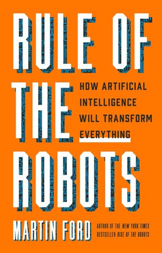
Rule of the Robots: How Artificial Intelligence Will Transform Everything
by
Martin Ford
Published 13 Sep 2021
Tuning the weights so the network eventually succeeds in converging on the right answer nearly every time is where the famous backpropagation algorithm comes in. A complex deep learning system might have a billion or more connections between neurons, each of which has a weight that needs to be optimized. Backpropagation essentially allows all the weights in the network to be adjusted collectively, rather than one at a time, delivering a massive boost to computational efficiency.1 During the training process, the output from the network is compared to the correct answer, and information that allows each weight to be adjusted accordingly propagates back through the layers of neurons. Without backpropagation, the deep learning revolution would not have been possible.
…
In the early 1980s, David Rumelhart, a psychology professor at the University of California, San Diego, conceived the technique known as “backpropagation,” which is still the primary learning algorithm used in multilayered neural networks today. Rumelhart, along with Ronald Williams, a computer scientist at Northeastern University, and Geoffrey Hinton, then at Carnegie Mellon, described how the algorithm could be used in what is now considered to be one of the most important scientific papers in artificial intelligence, published in the journal Nature in 1986.10 Backpropagation represented the fundamental conceptual breakthrough that would someday lead deep learning to dominate the field of AI, but it would be decades before computers would become fast enough to truly leverage the approach.
…
Geoffrey Hinton, who had been a young postdoctoral researcher working with Rumelhart at UC San Diego in 1981,11 would go on to become perhaps the most prominent figure in the deep learning revolution. By the end of the 1980s, practical applications for neural networks began to emerge. Yann LeCun, then a researcher at AT&T’s Bell Labs, used the backpropagation algorithm in a new architecture called a “convolutional neural network.” In convolutional networks, the artificial neurons are connected in a way that is inspired by the visual cortex in the brains of mammals, and these networks were designed to be especially effective at image recognition. LeCun’s system could recognize handwritten digits, and by the late 1990s convolutional neural networks were allowing ATM machines to understand the numbers written on bank checks.
Talk to Me: How Voice Computing Will Transform the Way We Live, Work, and Think
by
James Vlahos
Published 1 Mar 2019
It adjusts their numerical values, moving them closer to getting things right. Then backpropagation moves down to the next layer (the cheese) and does the same thing. The process repeats, continuing in reverse order, for any prior hidden layers (the meats). Backpropagation doesn’t work all at once. Depending on the complexity of the problem, the process might require millions of passes through the stack of layers, with tiny numerical adjustments to the outputs and weights happening each time. But by the end, the network will have automatically configured itself to produce correct answers. The importance of backpropagation can’t be overstated; virtually all of today’s neural networks have this simple algorithm as their backbone.
…
With machine learning, machines are supposed to learn—and in the early 1980s, it was David Rumelhart, assisted by Hinton and Ronald Williams, who ingeniously figured out a way to make that happen. Their solution was to employ a learning algorithm called backpropagation. Imagine showing a circle to that hypothetical image-recognition system we have been discussing. The first time you did that, all of the numerical values—the outputs of the individual neurons and the adjustment weights between them—would be totally off. The system would spit out a wrong answer. So then you manually set the output layer to have the right answer: a circle. From here, backpropagation works its mathematical magic. Working backward as the name suggests, the algorithm looks at the final hidden layer (call it the lettuce in the sandwich) and assesses how much each individual neuron contributed to the wrong answer.
…
But when Rumelhart, Hinton, and Williams published a landmark paper about the technique in 1986, the celebratory confetti didn’t rain down. The problem was that while backpropagation was intriguing in theory, actual demonstrations of neural networks powered by the technique were scarce and underwhelming. Here’s where Yann LeCun and Yoshua Bengio enter the picture. Those historic Perceptron experiments had been one of LeCun’s original inspirations for pursuing AI, and as a researcher in Hinton’s lab in the late 1980s, LeCun worked on backpropagation. Then, as a researcher at AT&T Bell Laboratories, he met Bengio, and the two would give neural networks what they badly needed: a success story.
Data Mining: Concepts, Models, Methods, and Algorithms
by
Mehmed Kantardzić
Published 2 Jan 2003
A graph of a multilayered-perceptron architecture with two hidden layers. MLPs have been applied successfully to solve some difficult and diverse problems by training the network in a supervised manner with a highly popular algorithm known as the error backpropagation algorithm. This algorithm is based on the error-correction learning rule and it may be viewed as its generalization. Basically, error backpropagation learning consists of two phases performed through the different layers of the network: a forward pass and a backward pass. In the forward pass, a training sample (input data vector) is applied to the input nodes of the network, and its effect propagates through the network layer by layer.
…
The backward procedure is repeated until all layers are covered and all weight factors in the network are modified. Then, the backpropagation algorithm continues with a new training sample. When there are no more training samples, the first iteration of the learning process finishes. With the same samples, it is possible to go through a second, third, and sometimes hundreds of iterations until error energy Eav for the given iteration is small enough to stop the algorithm. The backpropagation algorithm provides an “approximation” to the trajectory in weight space computed by the method of steepest descent.
…
(www.kxen.com) KXEN (Knowledge eXtraction ENgines), providing Vapnik SVM (Support Vector Machines) tools, including data preparation, segmentation, time series, and SVM classifiers. NeuroSolutions Vendor: NeuroDimension Inc. (www.neurosolutions.com) NeuroSolutions combines a modular, icon-based network design interface with an implementation of advanced learning procedures, such as recurrent backpropagation and backpropagation through time, and it solves data-mining problems such as classification, prediction, and function approximation. Some other notable features include C++ source code generation, customized components through DLLs, a comprehensive macro language, and Visual Basic accessibility through OLE Automation.
Hands-On Machine Learning With Scikit-Learn and TensorFlow: Concepts, Tools, and Techniques to Build Intelligent Systems
by
Aurélien Géron
Published 13 Mar 2017
Okay, now you know how to build an RNN network (or more precisely an RNN network unrolled through time). But how do you train it? Training RNNs To train an RNN, the trick is to unroll it through time (like we just did) and then simply use regular backpropagation (see Figure 14-5). This strategy is called backpropagation through time (BPTT). Figure 14-5. Backpropagation through time Just like in regular backpropagation, there is a first forward pass through the unrolled network (represented by the dashed arrows); then the output sequence is evaluated using a cost function (where tmin and tmax are the first and last output time steps, not counting the ignored outputs), and the gradients of that cost function are propagated backward through the unrolled network (represented by the solid arrows); and finally the model parameters are updated using the gradients computed during BPTT.
…
Now, if you want your neural network to predict housing prices like in Chapter 2, then you need one output neuron, using no activation function at all in the output layer.4 Backpropagation is a technique used to train artificial neural networks. It first computes the gradients of the cost function with regards to every model parameter (all the weights and biases), and then it performs a Gradient Descent step using these gradients. This backpropagation step is typically performed thousands or millions of times, using many training batches, until the model parameters converge to values that (hopefully) minimize the cost function. To compute the gradients, backpropagation uses reverse-mode autodiff (although it wasn’t called that when backpropagation was invented, and it has been reinvented several times).
…
Pac-Man Using Deep Q-Learning actual class, Confusion Matrix AdaBoost, AdaBoost-AdaBoost Adagrad, AdaGrad-AdaGrad Adam optimization, Faster Optimizers, Adam Optimization-Adam Optimization adaptive learning rate, AdaGrad adaptive moment optimization, Adam Optimization agents, Learning to Optimize Rewards AlexNet architecture, AlexNet-AlexNet algorithmspreparing data for, Prepare the Data for Machine Learning Algorithms-Select and Train a Model AlphaGo, Reinforcement Learning, Introduction to Artificial Neural Networks, Reinforcement Learning, Policy Gradients Anaconda, Create the Workspace anomaly detection, Unsupervised learning Apple’s Siri, Introduction to Artificial Neural Networks apply_gradients(), Gradient Clipping, Policy Gradients area under the curve (AUC), The ROC Curve arg_scope(), Implementing Batch Normalization with TensorFlow array_split(), Incremental PCA artificial neural networks (ANNs), Introduction to Artificial Neural Networks-ExercisesBoltzmann Machines, Boltzmann Machines-Boltzmann Machines deep belief networks (DBNs), Deep Belief Nets-Deep Belief Nets evolution of, From Biological to Artificial Neurons Hopfield Networks, Hopfield Networks-Hopfield Networks hyperparameter fine-tuning, Fine-Tuning Neural Network Hyperparameters-Activation Functions overview, Introduction to Artificial Neural Networks-From Biological to Artificial Neurons Perceptrons, The Perceptron-Multi-Layer Perceptron and Backpropagation self-organizing maps, Self-Organizing Maps-Self-Organizing Maps training a DNN with TensorFlow, Training a DNN Using Plain TensorFlow-Using the Neural Network artificial neuron, Logical Computations with Neurons(see also artificial neural network (ANN)) assign(), Manually Computing the Gradients association rule learning, Unsupervised learning associative memory networks, Hopfield Networks assumptions, checking, Check the Assumptions asynchronous updates, Asynchronous updates-Asynchronous updates asynchrous communication, Asynchronous Communication Using TensorFlow Queues-PaddingFifoQueue atrous_conv2d(), ResNet attention mechanism, An Encoder–Decoder Network for Machine Translation attributes, Supervised learning, Take a Quick Look at the Data Structure-Take a Quick Look at the Data Structure(see also data structure) combinations of, Experimenting with Attribute Combinations-Experimenting with Attribute Combinations preprocessed, Take a Quick Look at the Data Structure target, Take a Quick Look at the Data Structure autodiff, Using autodiff-Using autodiff, Autodiff-Reverse-Mode Autodiffforward-mode, Forward-Mode Autodiff-Forward-Mode Autodiff manual differentiation, Manual Differentiation numerical differentiation, Numerical Differentiation reverse-mode, Reverse-Mode Autodiff-Reverse-Mode Autodiff symbolic differentiation, Symbolic Differentiation-Numerical Differentiation autoencoders, Autoencoders-Exercisesadversarial, Other Autoencoders contractive, Other Autoencoders denoising, Denoising Autoencoders-TensorFlow Implementation efficient data representations, Efficient Data Representations generative stochastic network (GSN), Other Autoencoders overcomplete, Unsupervised Pretraining Using Stacked Autoencoders PCA with undercomplete linear autoencoder, Performing PCA with an Undercomplete Linear Autoencoder reconstructions, Efficient Data Representations sparse, Sparse Autoencoders-TensorFlow Implementation stacked, Stacked Autoencoders-Unsupervised Pretraining Using Stacked Autoencoders stacked convolutional, Other Autoencoders undercomplete, Efficient Data Representations variational, Variational Autoencoders-Generating Digits visualizing features, Visualizing Features-Visualizing Features winner-take-all (WTA), Other Autoencoders automatic differentiating, Up and Running with TensorFlow autonomous driving systems, Recurrent Neural Networks Average Absolute Deviation, Select a Performance Measure average pooling layer, Pooling Layer avg_pool(), Pooling Layer B backpropagation, Multi-Layer Perceptron and Backpropagation-Multi-Layer Perceptron and Backpropagation, Vanishing/Exploding Gradients Problems, Unsupervised Pretraining, Visualizing Features backpropagation through time (BPTT), Training RNNs bagging and pasting, Bagging and Pasting-Out-of-Bag Evaluationout-of-bag evaluation, Out-of-Bag Evaluation-Out-of-Bag Evaluation in Scikit-Learn, Bagging and Pasting in Scikit-Learn-Bagging and Pasting in Scikit-Learn bandwidth saturation, Bandwidth saturation-Bandwidth saturation BasicLSTMCell, LSTM Cell BasicRNNCell, Distributing a Deep RNN Across Multiple GPUs-Distributing a Deep RNN Across Multiple GPUs Batch Gradient Descent, Batch Gradient Descent-Batch Gradient Descent, Lasso Regression batch learning, Batch learning-Batch learning Batch Normalization, Batch Normalization-Implementing Batch Normalization with TensorFlow, ResNetoperation summary, Batch Normalization with TensorFlow, Implementing Batch Normalization with TensorFlow-Implementing Batch Normalization with TensorFlow batch(), Other convenience functions batch_join(), Other convenience functions batch_norm(), Implementing Batch Normalization with TensorFlow-Implementing Batch Normalization with TensorFlow Bellman Optimality Equation, Markov Decision Processes between-graph replication, In-Graph Versus Between-Graph Replication bias neurons, The Perceptron bias term, Linear Regression bias/variance tradeoff, Learning Curves biases, Construction Phase binary classifiers, Training a Binary Classifier, Logistic Regression biological neurons, From Biological to Artificial Neurons-Biological Neurons black box models, Making Predictions blending, Stacking-Exercises Boltzmann Machines, Boltzmann Machines-Boltzmann Machines(see also restricted Boltzman machines (RBMs)) boosting, Boosting-Gradient BoostingAdaBoost, AdaBoost-AdaBoost Gradient Boosting, Gradient Boosting-Gradient Boosting bootstrap aggregation (see bagging) bootstrapping, Grid Search, Bagging and Pasting, Introduction to OpenAI Gym, Learning to Play Ms.
Programming Collective Intelligence
by
Toby Segaran
Published 17 Dec 2008
, Crawler Code, Setting Up the Schema createindextables function, Setting Up the Schema distancescore function, Word Distance frequencyscore function, Normalization Function getentryid function, Adding to the Index getmatchrows function, Querying gettextonly function, Finding the Words on a Page import statements, Crawler Code importing neural network, Training Test inboundlinkscore function, Using Inbound Links isindexed function, Building the Index, Adding to the Index linktextscore function, Using the Link Text normalization function, Normalization Function searcher class, Content-Based Ranking, Training Test, Exercises nnscore function, Exercises query method, Training Test searchnet class, Training with Backpropagation, Training with Backpropagation, Training with Backpropagation backPropagate function, Training with Backpropagation trainquery method, Training with Backpropagation updatedatabase method, Training with Backpropagation separatewords function, Finding the Words on a Page searchindex.db, Setting Up the Schema, Adding to the Index searching, random, Random Searching self-organizing maps, Supervised versus Unsupervised Learning sigmoid function, Feeding Forward signups, predicting, Predicting Signups simulated annealing, Simulated Annealing, The Cost Function socialnetwork.py, The Layout Problem, Counting Crossed Lines, Drawing the Network crosscount function, Counting Crossed Lines drawnetwork function, Drawing the Network spam filtering, Limits of Machine Learning, Filtering Spam, Choosing a Category, Choosing a Category method, Limits of Machine Learning threshold, Choosing a Category tips, Choosing a Category SpamBayes plug-in, The Fisher Method spidering, A Simple Crawler SQLite, Building the Index, Setting Up the Schema, Persisting the Trained Classifiers, Installation on All Platforms embedded database interface, Installation on All Platforms persisting trained classifiers, Persisting the Trained Classifiers tables, Setting Up the Schema squaring numbers, Cross-Validation stemming algorithm, Adding to the Index stochastic optimization, Optimization stock market analysis, Other Uses for Learning Algorithms stock market data, Using Stock Market Data, Using Stock Market Data, What Is Trading Volume?
…
, Mutating Programs N naïve Bayesian classifier, A Naïve Classifier, Choosing a Category, The Fisher Method, Classifying, Strengths and Weaknesses choosing category, Choosing a Category strengths and weaknesses, Strengths and Weaknesses versus Fisher method, The Fisher Method national security, Other Uses for Learning Algorithms nested dictionary, Collecting Preferences Netflix, Introduction to Collective Intelligence, Real-Life Examples network visualization, Network Visualization, Counting Crossed Lines, Drawing the Network counting crossed lines, Counting Crossed Lines drawing networks, Drawing the Network layout problem, Network Visualization network vizualization, Network Visualization neural network, What's in a Search Engine?, Learning from Clicks, Learning from Clicks, Setting Up the Database, Feeding Forward, Training with Backpropagation, Training Test, Training Test artificial, Learning from Clicks, Learning from Clicks, Setting Up the Database, Feeding Forward, Training with Backpropagation, Training Test, Training Test backpropagation, Training with Backpropagation connecting to search engine, Training Test designing click-training network, Learning from Clicks feeding forward, Feeding Forward setting up database, Setting Up the Database training test, Training Test neural network classifier, Exercises neural networks, Neural Networks, Neural Networks, Neural Networks, Neural Networks, Training a Neural Network, Training a Neural Network, Training a Neural Network, Strengths and Weaknesses, Strengths and Weaknesses backpropagation, and, Training a Neural Network black box method, Strengths and Weaknesses combinations of words, and, Neural Networks multilayer perceptron network, Neural Networks strengths and weaknesses, Strengths and Weaknesses synapses, and, Neural Networks training, Training a Neural Network using code, Training a Neural Network news sources, A Corpus of News newsfeatures.py, Selecting Sources, Downloading Sources, Downloading Sources, Downloading Sources, Converting to a Matrix, Using NumPy, The Algorithm, Displaying the Results, Displaying the Results, Displaying by Article, Displaying by Article getarticlewords function, Downloading Sources makematrix function, Converting to a Matrix separatewords function, Downloading Sources shape function, The Algorithm showarticles function, Displaying the Results, Displaying by Article showfeatures function, Displaying the Results, Displaying by Article stripHTML function, Downloading Sources transpose function, Using NumPy nn.py, Setting Up the Database, Setting Up the Database, Setting Up the Database, Setting Up the Database searchnet class, Setting Up the Database, Setting Up the Database, Setting Up the Database, Setting Up the Database generatehiddennode function, Setting Up the Database getstrength method, Setting Up the Database setstrength method, Setting Up the Database nnmf.py, The Algorithm difcost function, The Algorithm non-negative matrix factorization (NMF), Supervised versus Unsupervised Learning, Clustering, Non-Negative Matrix Factorization, Non-Negative Matrix Factorization, Non-Negative Matrix Factorization, Using Your NMF Code factorization, Supervised versus Unsupervised Learning goal of, Non-Negative Matrix Factorization update rules, Non-Negative Matrix Factorization using code, Using Your NMF Code normalization, Normalization Function numerical predictions, Building Price Models numpredict.py, Building a Sample Dataset, Building a Sample Dataset, Defining Similarity, Defining Similarity, Defining Similarity, Defining Similarity, Subtraction Function, Subtraction Function, Weighted kNN, Weighted kNN, Cross-Validation, Cross-Validation, Cross-Validation, Heterogeneous Variables, Scaling Dimensions, Optimizing the Scale, Optimizing the Scale, Uneven Distributions, Estimating the Probability Density, Graphing the Probabilities, Graphing the Probabilities, Graphing the Probabilities createcostfunction function, Optimizing the Scale createhiddendataset function, Uneven Distributions crossvalidate function, Cross-Validation, Optimizing the Scale cumulativegraph function, Graphing the Probabilities distance function, Defining Similarity dividedata function, Cross-Validation euclidian function, Defining Similarity gaussian function, Weighted kNN getdistances function, Defining Similarity inverseweight function, Subtraction Function knnestimate function, Defining Similarity probabilitygraph function, Graphing the Probabilities probguess function, Estimating the Probability Density, Graphing the Probabilities rescale function, Scaling Dimensions subtractweight function, Subtraction Function testalgorithm function, Cross-Validation weightedknn function, Weighted kNN wineprice function, Building a Sample Dataset wineset1 function, Building a Sample Dataset wineset2 function, Heterogeneous Variables NumPy, Using NumPy, Using NumPy, Simple Usage Example, NumPy, Installation on Other Platforms, Installation on Other Platforms installation on other platforms, Installation on Other Platforms installation on Windows, Simple Usage Example usage example, Installation on Other Platforms using, Using NumPy O online technique, Strengths and Weaknesses Open Web APIs, Open APIs optimization, Optimization, Group Travel, Representing Solutions, Representing Solutions, Representing Solutions, Representing Solutions, The Cost Function, The Cost Function, The Cost Function, Random Searching, Hill Climbing, Simulated Annealing, Genetic Algorithms, Genetic Algorithms, Genetic Algorithms, Genetic Algorithms, Genetic Algorithms, Genetic Algorithms, Optimizing for Preferences, Optimizing for Preferences, The Cost Function, The Cost Function, Network Visualization, Network Visualization, Counting Crossed Lines, Drawing the Network, Exercises, Exercises, Exercises, Exercises, Exercises, Exercises, Exercises, Optimizing the Scale, Exercises, Optimization, Optimization annealing starting points, Exercises cost function, The Cost Function, Optimization exercises, Exercises genetic algorithms, Genetic Algorithms, Genetic Algorithms, Genetic Algorithms, Genetic Algorithms, Genetic Algorithms crossover or breeding, Genetic Algorithms generation, Genetic Algorithms mutation, Genetic Algorithms population, Genetic Algorithms genetic optimization stopping criteria, Exercises group travel cost function, Exercises group travel planning, Group Travel, Representing Solutions, Representing Solutions, Representing Solutions, The Cost Function, The Cost Function car rental period, The Cost Function departure time, Representing Solutions price, Representing Solutions time, Representing Solutions waiting time, The Cost Function hill climbing, Hill Climbing line angle penalization, Exercises network visualization, Network Visualization, Counting Crossed Lines, Drawing the Network counting crossed lines, Counting Crossed Lines drawing networks, Drawing the Network layout problem, Network Visualization network vizualization, Network Visualization pairing students, Exercises preferences, Optimizing for Preferences, Optimizing for Preferences, The Cost Function, The Cost Function cost function, The Cost Function running, The Cost Function student dorm, Optimizing for Preferences random searching, Random Searching representing solutions, Representing Solutions round-trip pricing, Exercises simulated annealing, Simulated Annealing where it may not work, Genetic Algorithms optimization.py, Group Travel, Representing Solutions, Representing Solutions, The Cost Function, Random Searching, Hill Climbing, Simulated Annealing, Genetic Algorithms, Genetic Algorithms, Genetic Algorithms, Genetic Algorithms, Genetic Algorithms, Optimizing the Scale annealingoptimize function, Simulated Annealing geneticoptimize function, Genetic Algorithms, Genetic Algorithms, Genetic Algorithms, Genetic Algorithms, Genetic Algorithms elite, Genetic Algorithms maxiter, Genetic Algorithms mutprob, Genetic Algorithms popsize, Genetic Algorithms getminutes function, Representing Solutions hillclimb function, Hill Climbing printschedule function, Representing Solutions randomoptimize function, Random Searching schedulecost function, The Cost Function P PageRank algorithm, Real-Life Examples, The PageRank Algorithm pairing students, Exercises Pandora, Real-Life Examples parse tree, Programs As Trees Pearson correlation, Hierarchical Clustering, Viewing Data in Two Dimensions hierarchical clustering, Hierarchical Clustering multidimensional scaling, Viewing Data in Two Dimensions Pearson correlation coefficient, Pearson Correlation Score, Pearson Correlation Coefficient, Pearson Correlation Coefficient code, Pearson Correlation Coefficient Pilgrim, Mark, Universal Feed Parser polynomial transformation, The Kernel Trick poplib, Exercises population, Genetic Algorithms, What Is Genetic Programming?
…
, Crawler Code, Crawler Code, Building the Index, Setting Up the Schema, Setting Up the Schema, Finding the Words on a Page, Finding the Words on a Page, Adding to the Index, Adding to the Index, Adding to the Index, Querying, Content-Based Ranking, Normalization Function, Normalization Function, Word Distance, Using Inbound Links, Using the Link Text, Training with Backpropagation, Training with Backpropagation, Training with Backpropagation, Training Test, Training Test, Exercises addtoindex function, Adding to the Index crawler class, What's in a Search Engine?, Crawler Code, Setting Up the Schema createindextables function, Setting Up the Schema distancescore function, Word Distance frequencyscore function, Normalization Function getentryid function, Adding to the Index getmatchrows function, Querying gettextonly function, Finding the Words on a Page import statements, Crawler Code importing neural network, Training Test inboundlinkscore function, Using Inbound Links isindexed function, Building the Index, Adding to the Index linktextscore function, Using the Link Text normalization function, Normalization Function searcher class, Content-Based Ranking, Training Test, Exercises nnscore function, Exercises query method, Training Test searchnet class, Training with Backpropagation, Training with Backpropagation, Training with Backpropagation backPropagate function, Training with Backpropagation trainquery method, Training with Backpropagation updatedatabase method, Training with Backpropagation separatewords function, Finding the Words on a Page searchindex.db, Setting Up the Schema, Adding to the Index searching, random, Random Searching self-organizing maps, Supervised versus Unsupervised Learning sigmoid function, Feeding Forward signups, predicting, Predicting Signups simulated annealing, Simulated Annealing, The Cost Function socialnetwork.py, The Layout Problem, Counting Crossed Lines, Drawing the Network crosscount function, Counting Crossed Lines drawnetwork function, Drawing the Network spam filtering, Limits of Machine Learning, Filtering Spam, Choosing a Category, Choosing a Category method, Limits of Machine Learning threshold, Choosing a Category tips, Choosing a Category SpamBayes plug-in, The Fisher Method spidering, A Simple Crawler SQLite, Building the Index, Setting Up the Schema, Persisting the Trained Classifiers, Installation on All Platforms embedded database interface, Installation on All Platforms persisting trained classifiers, Persisting the Trained Classifiers tables, Setting Up the Schema squaring numbers, Cross-Validation stemming algorithm, Adding to the Index stochastic optimization, Optimization stock market analysis, Other Uses for Learning Algorithms stock market data, Using Stock Market Data, Using Stock Market Data, What Is Trading Volume?
Mastering Machine Learning With Scikit-Learn
by
Gavin Hackeling
Published 31 Oct 2014
It is given by the following equation, where m is the number of training instances: MSE = 2 1 m ( yi − f ( xi ) ) ∑ m i =1 Minimizing the cost function The backpropagation algorithm is commonly used in conjunction with an optimization algorithm such as gradient descent to minimize the value of the cost function. The algorithm takes its name from a portmanteau of backward propagation, and refers to the direction in which errors flow through the layers of the network. Backpropagation can theoretically be used to train a feedforward network with any number of hidden units arranged in any number of layers, though computational power constrains this capability. Backpropagation is similar to gradient descent in that it uses the gradient of the cost function to update the values of the model parameters.
…
If a random change to one of the weights decreases the value of the cost function, we save the change and randomly change the value of another weight. An obvious problem with this solution is its prohibitive computational cost. Backpropagation provides a more efficient solution. [ 191 ] www.it-ebooks.info From the Perceptron to Artificial Neural Networks We will step through training a feedforward neural network using backpropagation. This network has two input units, two hidden layers that both have three hidden units, and two output units. The input units are both fully connected to the first hidden layer's units, called Hidden1, Hidden2, and Hidden3.
…
We can now perform another forward pass using the new values of the weights; the value of the cost function produced using the updated weights should be smaller. We will repeat this process until the model converges or another stopping criterion is satisfied. Unlike the linear models we have discussed, backpropagation does not optimize a convex function. It is possible that backpropagation will converge on parameter values that specify a local, rather than global, minimum. In practice, local optima are frequently adequate for many applications. [ 211 ] www.it-ebooks.info From the Perceptron to Artificial Neural Networks Approximating XOR with Multilayer perceptrons Let's train a multilayer perceptron to approximate the XOR function.
The Ethical Algorithm: The Science of Socially Aware Algorithm Design
by
Michael Kearns
and
Aaron Roth
Published 3 Oct 2019
Pseudocode for the backpropagation algorithm for neural networks. So when people talk about the complexity and opaqueness of machine learning, they really don’t (or at least shouldn’t) mean the actual optimization algorithms, such as backpropagation. These are the algorithms designed by human beings. But the models they produce—the outputs of such algorithms—can be complicated and inscrutable, especially when the input data is itself complex and the space of possible models is immense. And this is why the human being deploying the model won’t fully understand it. The goal of backpropagation is perfectly understandable: minimize the error on the input data.
…
The solid curve makes even fewer errors but is more complicated, potentially leading to unintended side effects. The standard and most widely used meta-algorithms in machine learning are simple, transparent, and principled. In Figure 2 we replicate the high-level description or “pseudocode” from Wikipedia for the famous backpropagation algorithm for neural networks, a powerful class of predictive models. This description is all of eleven lines long, and it is easily taught to undergraduates. The main “forEach” loop is simply repeatedly cycling through the data points (the positive and negative dots on the page) and adjusting the parameters of the model (the curve you were fitting) in an attempt to reduce the number of misclassifications (positive points the model misclassifies as negative, and negative points the model misclassifies as positive).
…
This worldview is actually shared by many computer scientists, not only the theoretical ones. The distinguishing feature of theoretical computer science is the desire to formulate mathematically precise models of computational phenomena and to explore their algorithmic consequences. A machine learning practitioner might develop or take an algorithm like backpropagation for neural networks, which we discussed earlier, and apply it to real data to see how well it performs. Doing so doesn’t really require the practitioner to precisely specify what “learning” means or doesn’t mean, or what computational difficulties it might present generally. She can simply see whether the algorithm works well for the specific data or task at hand.
The Alignment Problem: Machine Learning and Human Values
by
Brian Christian
Published 5 Oct 2020
The idea of reinforcement learning as “learning with a critic” appears to date back at least as far as Widrow, Gupta, and Maitra, “Punish/Reward.” 30. You can think of an algorithm like backpropagation as solving the credit-assignment problem structurally, rather than temporally. As Sutton put it in “Learning to Predict by the Methods of Temporal Differences,” “The purpose of both backpropagation and TD methods is accurate credit assignment. Backpropagation decides which part(s) of a network to change so as to influence the network’s output and thus to reduce its overall error, whereas TD methods decide how each output of a temporal sequence of outputs should be changed. Backpropagation addresses a structural credit-assignment issue whereas TD methods address a temporal credit-assignment issue.” 31.
…
Alex Krizhevsky, personal interview, June 12, 2019. 12. The method for determining the gradient update in a deep network is known as “backpropagation”; it is essentially the chain rule from calculus, although it requires the use of differentiable neurons, not the all-or-nothing neurons considered by McCulloch, Pitts, and Rosenblatt. The work that popularized the technique is considered to be Rumelhart, Hinton, and Williams, “Learning Internal Representations by Error Propagation,” although backpropagation has a long history that dates back to the 1960s and ’70s, and important advances in training deep networks have continued to emerge in the twenty-first century. 13.
…
For seminal papers relating to Bayesian neural networks, see Denker et al., “Large Automatic Learning, Rule Extraction, and Generalization”; Denker and LeCun, “Transforming Neural-Net Output Levels to Probability Distributions”; MacKay, “A Practical Bayesian Framework for Backpropagation Networks”; Hinton and Van Camp, “Keeping Neural Networks Simple by Minimizing the Description Length of the Weights”; Neal, “Bayesian Learning for Neural Networks”; and Barber and Bishop, “Ensemble Learning in Bayesian Neural Networks.” For more recent work, see Graves, “Practical Variational Inference for Neural Networks”; Blundell et al., “Weight Uncertainty in Neural Networks”; and Hernández-Lobato and Adams, “Probabilistic Backpropagation for Scalable Learning of Bayesian Neural Networks.” For a more detailed history of these ideas, see Gal, “Uncertainty in Deep Learning.”
Machine, Platform, Crowd: Harnessing Our Digital Future
by
Andrew McAfee
and
Erik Brynjolfsson
Published 26 Jun 2017
Byrne, “Introduction to Neurons and Neuronal Networks,” Neuroscience Online, accessed January 26, 2017, http://neuroscience.uth.tmc.edu/s1/introduction.html. 73 “the embryo of an electronic computer”: Mikel Olazaran, “A Sociological Study of the Official History of the Perceptrons Controversy,” Social Studies of Science 26 (1996): 611–59, http://journals.sagepub.com/doi/pdf/10.1177/030631296026003005. 74 Paul Werbos: Jürgen Schmidhuber, “Who Invented Backpropagation?” last modified 2015, http://people.idsia.ch/~juergen/who-invented-backpropagation.html. 74 Geoff Hinton: David E. Rumelhart, Geoffrey E. Hinton, and Ronald J. Williams, “Learning Representations by Back-propagating Errors,” Nature 323 (1986): 533–36, http://www.nature.com/nature/journal/v323/n6088/abs/323533a0.html. 74 Yann LeCun: Jürgen Schmidhuber, Deep Learning in Neural Networks: An Overview, Technical Report IDSIA-03-14, October 8, 2014, https://arxiv.org/pdf/1404.7828v4.pdf. 74 as many as 20% of all handwritten checks: Yann LeCun, “Biographical Sketch,” accessed January 26, 2017, http://yann.lecun.com/ex/bio.html. 74 “a new approach to computer Go”: David Silver et al., “Mastering the Game of Go with Deep Neural Networks and Search Trees,” Nature 529 (2016): 484–89, http://www.nature.com/nature/journal/v529/n7587/full/nature16961.html. 75 approximately $13,000 by the fall of 2016: Elliott Turner, Twitter post, September 30, 2016 (9:18 a.m.), https://twitter.com/eturner303/status/781900528733261824. 75 “the teams at the leading edge”: Andrew Ng, interview by the authors, August 2015. 76 “Retrospectively, [success with machine learning]”: Paul Voosen, “The Believers,” Chronicle of Higher Education, February 23, 2015, http://www.chronicle.com/article/The-Believers/190147. 76 His 2006 paper: G.
…
They did this with a combination of sophisticated math, ever-more-powerful computer hardware, and a pragmatic approach that allowed them to take inspiration from how the brain works but not to be constrained by it. Electric signals flow in only one direction through the brain’s neurons, for example, but the successful machine learning systems built in the eighties by Paul Werbos, Geoff Hinton, Yann LeCun, and others allowed information to travel both forward and backward through the network. This “back-propagation” led to much better performance, but progress remained frustratingly slow. By the 1990s, a machine learning system developed by LeCun to recognize numbers was reading as many as 20% of all handwritten checks in the United States, but there were few other real-world applications. As AlphaGo’s recent victory shows, the situation is very different now.
The Long History of the Future: Why Tomorrow's Technology Still Isn't Here
by
Nicole Kobie
Published 3 Jul 2024
In particular, no one could figure out how to train such a complicated system, or how to adjust the weights.13 Finding the answer was what made neural networks possible. Backpropagation works from the output back to the input, adjusting the weights as it goes, with the aim of shrinking the difference between what the network initially outputted and a defined desired output. It’s unclear who first originated this idea, though it may well have been invented at multiple different times. In 1974, Paul Werbos published his dissertation explaining how to use backpropagation of errors to train neural networks, though his work was little noticed until 1986 when it was cited in a paper by Rumelhart, Ronald Williams and Geoffrey Hinton, the latter now considered one of the ‘fathers of deep learning’.
…
None of those points are currently considered, and even if they were, we don’t have the data points to fill those inputs. There are various techniques to boost the accuracy of a model in training, including reinforcement learning, which is when a system learns through trial and error; cost functions, which compare the model’s outputs with what they should be; and ideas like backpropagation, which involves automatically going back in an algorithm to figure out where mistakes are being made in order to fix them. Inaccuracies can be caused by incorrect weights, misaligned thresholds and simple bad data – if there actually are sharks in the water, that would be a troubling problem to find out once on your surfboard.
…
Deep learning is powered by neural networks, and there’s a variety of different types, including convolutional neural networks, which analyse data such as images by starting at very basic features such as brightness before zooming in to higher resolution; and recurrent neural networks, which have memory so can go back and examine earlier pieces of data for better context, making them helpful for language and so on. Different algorithm types are useful for different tasks. Developing these systems and figuring out backpropagation is one part of the ‘maths problem’, and Hinton and other researchers carried on toiling away at deep learning when everyone else got distracted – he and the rest have been repaid marvellously for such dedication, as is only right. * * * Another problem is data, which was initially solved by Fei-Fei Li, director of the Stanford Artificial Intelligence Lab and co-founder of the Stanford Institute for Human-Centred Artificial Intelligence (HAI).
Rationality: What It Is, Why It Seems Scarce, Why It Matters
by
Steven Pinker
Published 14 Oct 2021
The challenge in getting these networks to work is how to train them. The problem is with the connections from the input layer to the hidden layer: since the units are hidden from the environment, their guesses cannot be matched against “correct” values supplied by the teacher. But a breakthrough in the 1980s, the error back-propagation learning algorithm, cracked the problem.32 First, the mismatch between each output unit’s guess and the correct answer is used to tweak the weights of the hidden-to-output connections in the top layer, just like in the simple networks. Then the sum of all these errors is propagated backwards to each hidden unit to tweak the input-to-hidden connections in the middle layer.
…
Global, regional, and national age-sex-specific mortality for 282 causes of death in 195 countries and territories, 1980–2017: A systematic analysis for the Global Burden of Disease Study 2017. The Lancet, 392, 1736–88. https://doi.org/10.1016/S0140-6736(18)32203-7. Rumelhart, D. E., Hinton, G. E., & Williams, R. J. 1986. Learning representations by back-propagating errors. Nature, 323, 533–36. https://doi.org/10.1038/323533a0. Rumelhart, D. E., McClelland, J. L., & PDP Research Group. 1986. Parallel distributed processing: Explorations in the microstructure of cognition, vol. 1, Foundations. Cambridge, MA: MIT Press. Rumney, P. N. S. 2006. False allegations of rape.
…
See left and right (political) consistency, 82 conspiracy theories adherents of, equivocal, 298–99 beliefs in, not based on truth of, 302 COVID-19, 283–84 as entertainment, 303, 308 and evolution of ideas, 308–9 openness to evidence vs., 311 police, reporting to, 299, 308 popularity of, 286 as predating social media, 287 real conspiracies and, 307–8 reflective vs. intuitive, 299 rumor and, 308 signal detection and, 307–8 consumers extended warranties, 197–98 as money pumps, 176, 180, 185, 187–88 contradiction, anything follows from, 81–82 conventions and standards, 234–35 conversation, rules of, 10, 21, 28, 30, 78–80, 87–88, 308, 343n43 cooperation in the Prisoner’s Dilemma, 239–42 in Public Goods games, 242–44 coordination games, 233–35 correlation causation not implied by, 245–47, 251–52, 312, 321, 323–24, 329–30 coefficient (r), 250–51 cross-lagged panel correlation, 269–70 definition, 247 definition of “prediction,” 247 illusory, 245–46, 251–52, 321 San people and, 4 scatterplots, 247–52, 270–71 See also causation; regression Cosmides, L., 169 counterfactuals, 64, 257, 259, 264 heretical, 64–65 COVID-19, 2, 193–94, 242, 283 exponential growth bias and, 11–12 media fear mongering, 126–27 misinformation, 245, 283–84, 296, 316 Coyne, Jerry, 302 creationism, 173, 295, 305, 311 credit card debt, 11, 320–21 crib death, 129–30 Crick, Francis, 158 crime availability bias and perceptions of, 126 confirmation bias and, 13–14 Great American Crime Decline, 126 gun control and rates of, 292–93 and punishment, 332–33 rational ignorance and, 58 regression to the mean and, 255–56 signal detection and, 202, 216–21, 352n17 statistical independence and, 129 See also homicide; judicial system critical race theory, 123 critical theory, 35–36 critical thinking, 34, 36, 40, 87, 287, 314, 320 definition, 74 San people and, 3–4 stereotypes and failures of, 19–20, 27 teaching, 82, 87, 314–15 The Crown (TV series), 303 CSI (TV show), 216 Cuban Missile Crisis, 236 d, 214–16, 218–21, 352n17 Darwin, Charles, 173 data, vs. anecdotes, xiv, 119–22, 125, 167, 300, 312, 314 data snooping, 145–46, 160 Dawes, Robyn, 175 Dawkins, Richard, 302, 308 Dean, James. See Rebel Without a Cause death, 196, 197, 304 death penalty, 221, 294, 311, 333 deductive logic, 73–84, 95–100, 102, 108–9 deep learning networks biases perpetuated by, 107, 165 the brain compared to, 107–9 definition, 102 error back-propagation and, 105–6 hidden layers of neurons in, 105–7 intuition as demystified by, 107–8 logical inference distinguished from, 107 terms for, 102 two-layer networks, 103–5 De Freitas, Julian, 343n46 demagogues, 125, 126 democracy checks and balances in, 41, 316, 317 corrosion of truth as undermining, 309 data as a public good and, 119 education and information access predicts, 330 and peace, 88, 264, 266, 269–72, 327 presumption of innocence in, 218 and risk literacy, importance of, 171 and science, trust in, 145 Trump and threats to, 126, 130–31, 284, 313 Democratic Party and Democrats COVID-19 conspiracy theories involving, 283 expressive rationality and, 298 politically motivated numeracy and, 292–94 See also left and right (political); politics Dennett, Daniel, 231, 302 denying the antecedent, 83, 294 denying the consequent, 80–81 deontic logic, 84 dependence among events conjunctions and, 128–31, 137 defined via conditional probability, 137 falsely assuming, 131 the “hot hand” in basketball and, 131–32 the judicial system and, 129–30 selection of events and, 132 voter fraud claims and, 130–31 depression, 276–77, 276, 280 Derrida, Jacques, 90 Descartes, René, 40 deterministic systems, 114 Dick, Philip K., 298 dieter’s fallacy, 101 digital media ideals of, 316 truth-serving measures needed by, 314, 316–17 Wikipedia, 316 See also media; social media Dilbert cartoons, 91, 112–13, 112, 117 DiMaggio, Joe, 147–48 discounting the future, 47–56, 320 discrimination, forbidden base rates and, 163–66 disenchantment of the world (Weber), 303 disjunction of events, probability of, 128, 132–34 disjunctions (or), definition, 77 disjunctive addition, 81 disjunctive syllogism, 81 distributions, statistical, 203–5 bell curve (normal or Gaussian), 204–5 bimodal, 204 fat-tailed, 204–5 Ditto, Peter, 293–94, 297 DNA as forensic technique, 216 domestic violence, 138–39 Dostoevsky, Fyodor, 289 Douglass, Frederic, 338–39 dread risk, 122 dreams, 13, 304 Dr.
Explaining Humans: What Science Can Teach Us About Life, Love and Relationships
by
Camilla Pang
Published 12 Mar 2020
This is thanks to its second crucial component: the feedback system. By comparing predicted and actual results, the network can calculate its estimated error, and then use our old friend gradient descent (turn to p. 139 for a reminder) to determine which of the weighted connections are most in error, and how they should be adjusted: a process called backpropagation (aka self-reflection). In other words, the neural network does something that humans are often bad at: it learns from its mistakes. In fact, it is hardwired to do so, without the emotional baggage that humans attach to their mistakes, using feedback as an intrinsic component of its quest to improve.
…
And it’s supported by a litany of Post-it Notes reminding me to pick up my socks, call my mum (twice) and not to wash the jeans that have £5 in the pocket. Remembering to remember things is largely a question of finding the right mechanisms to remind yourself. Forgetting to be afraid is more complex. But this is about the feedback loop and backpropagation as well. Because I know that smoke or bad smells won’t actually do me any harm, I can use that proven outcome to counterbalance the weighted connection that tells me to be afraid. I can try to update the inputs that condition how I respond to particular situations, by reassuring myself about a track record of outputs.
…
actin (proteins) 33, 34 adaptor proteins 38, 39–40, 43, 46 ADHD (attention deficit hyperactivity disorder) x, xiv, 44 acceptance of 29, 119, 196, 197 boredom and xi, 85, 87, 163 brainwaves and 98–100 childhood and 87 decision making and 17, 101, 141, 185 diagnosis of 92, 101 fear and 77, 85, 86 goals and 131, 133, 139 gradient descent and 139, 141 harmony/amplitude and 92–3, 93, 98–106, 102, 105 information processing and xi, 13, 98–9 insomnia and 70 learning rate and 141 memory and 185–6 overthinking and 16, 102 panic induced by 77 patience and 131, 133, 139, 225 reading and 163–5 superpower 29 time perception and 13, 98, 131, 133, 139, 141 affinities (single interactions) 183 ageing, human 148–9 agent-based modelling (ABM) 210–14, 215, 216, 219 algorithms, computer decision making and xii, 1–24, 8, 15, 128–30, 134, 138–41, 143, 146, 156–60, 158, 187, 188–93, 189, 195, 199, 202, 203–204 fuzzy logic and 156–60 gradient descent algorithm 125, 138–41, 143, 191 human mind and 1, 4 limitations of 3 neural networks and 187, 188–93, 189, 195, 198, 202, 203 supervised learning and 4, 6, 23 unstructured, ability to be 2 unsupervised learning and 4, 5, 6, 10, 18, 21 see also machine learning alienation 98 alpha keratins 32 alpha waves 98 amino acids 31–2 amplitude 90–95, 96, 99, 100–104 anxiety ADHD and see ADHD ASD and see ASD Asperger’s syndrome and see Asperger’s syndrome attacks 14, 70–71, 73, 83, 142 colour and 70–71, 73, 102, 127 crowds and 14, 70, 114–15, 121 decision making and 12, 14, 16, 20, 51–2, 59, 61, 81, 83, 142 fear/light and 70–71, 72–4, 74, 76, 77, 78–9, 80, 81, 82–5 GAD (generalized anxiety disorder) x–xi, 74, 197 goals and 124, 134, 135, 137, 138, 142–3 harmony and 98–9, 102, 108 information processing and xi, 83 loud noises and 70, 87, 198 memory and 186, 204 night terrors 70 order and 48, 51–2, 59, 61 smell and 12, 14, 70, 102, 127, 160, 164–5, 199, 201, 204 as a strength 29, 82–4, 142–3 superpower 29 texture and 70 arguments 38, 154, 156–60, 162, 183 artificial intelligence (AI) 3, 156, 186, 187, 188, 189, 215 ASD (autism spectrum disorder) acceptance of 197 Asperger’s syndrome and xiii–xiv Bayes’ theorem and 155 crowds and 115 decision making and 6, 10, 12, 16 empathy and 145 explained x–xi fear and 70–71, 77, 80, 85, 86 memory and 194 order and 50, 51–2, 58 superpower 29 Asperger’s syndrome xiii–xiv autism and xiii–xiv Bayes’ theorem and 151–2 clubbing/music festivals and 153, 201 empathy and 145 fear/light and 71–2 meeting people and 151 memory and 194–5 politeness and 206 atom Brownian motion and 112, 114 chemical bonds and/atomic compounds 165, 166, 167–71, 172, 173, 174, 176, 177, 178, 180, 181, 184 crowds and 107, 111, 112, 114 light and 75 autism see ASD (autism spectrum disorder) avidity 183 backpropagation 191, 199 Bayes’ theorem 151–6, 159, 162, 206 bee colonies 36 beta waves 98 bias 153, 160, 162, 192, 196, 197, 202, 204 bioinformatics 209, 220 blood sugar levels 38, 65 bonds, chemical 165–84 bond length 173 covalent 168, 169, 170, 171, 173, 182, 183, 184 electromagnetic force 175–6 evolution of over time 180–83 four fundamental forces 174–80, 179 gravitational force 174–5 hydrophobic effect 171–3 ionic 169–71, 170, 173, 176, 180, 181, 184 strong (nuclear) force 176–7 tan(x) curve and 163–5, 164 valency and 173–4 weak (nuclear) force 177–80, 182 boredom xi, 41, 85, 87, 158, 163, 186, 192 box thinking 5–12, 8, 17, 19–20, 23, 24 brainwaves 98–100 Brown, Robert 112 Brownian motion 112–14, 113, 115 cancer xii, 4, 45–7, 85, 118, 149, 219, 220 carbon dioxide 168 cars braking 157 driverless 189, 190–91, 202 category failure 22–3 cell signalling 37, 38–42 cellular evolution 146, 147–50, 148, 151 stem cells 146, 147–8, 148, 149, 150 chaos 13–15, 17, 21, 29, 48, 60 chemical bonds see bonds, chemical childhood: ADHD and 87–8 box thinking and 8, 10 fear and 83, 109, 121 neurodiversity at school 25–8 time perception and 126–8 tree thinking and 10, 21 Civilization V (video game) 108 compound, atomic 167–71, 172, 180, 181 conditional probability 153 conflict resolution 157 connecting with others 163–84 avidity and 183 chemical bonds and 165–84, 170 four fundamental forces and 174–80, 179 fraying and decomposing connections 180–84 tan(x) curve and 163–5, 164 see also bonds, chemical consensus behaviours, understanding and modelling 110–18 covalent bonds 168, 169, 170, 171, 173, 182, 183, 184 crowds 12, 14, 26, 70, 107–21, 113, 201 anxiety and 14, 70, 114–15, 121 atom and 107, 111, 112, 114 Brownian motion and 112, 113, 115 consensus and 110–18 decision making and 108, 110, 111, 112 differences/diversity and 111, 116–17, 118 diversity and 117–18 dust particle movement and 107–108, 111, 112, 113, 116 ergodic theory and 115–20 full stop and 107–108 individuality and 115–21 Newton’s second law (force = mass × acceleration) and 114 stereotypes and 117 random walk 113 stochastic (randomly occurring) process and 115–16 data inputs 190 dating 144, 207, 221–2 apps 161, 193 decision making box thinking and 5–12, 8, 17, 19–20, 24 crowds and 108, 110, 111, 112 equilibrium and 66, 67, 68, 69 error, learning to embrace 21–4 fear and 71, 81 feedback loop and 199, 202, 203–204 fuzzy logic and 146, 156–60, 158 game theory and 215–18, 220 goals and 128–30, 134, 137, 138–41, 142, 143, 191 gradient descent algorithm and 138–41, 143, 191 homology and 220 how to decide 17–21 machine learning and xii, 1–24, 128–30, 134, 138–41, 143, 146, 156–60, 158, 187, 188–93, 189, 195, 199, 202, 203–204 memory and 187, 199, 203–204 network theory and 134, 138 neural networks and 187, 188–93, 189, 195, 198, 202, 203 probability and 146 proteins and 28, 36, 37, 38, 39, 42, 43, 46 tree, thinking like a and 5–7, 10–24, 15 deep learning 187, 188, 189–90 see also neural networks delta waves 98 denial 78, 83–4 depression 100–103 differences/diversity, understanding/ respecting 25–47, 226 cancer and 45–7, 118 chemical bonds and 165–6, 168, 169–71, 181–3 collaboration/success and 45–7 crowds and 111, 116–17, 118 empathy and 149 ergodicity and 118, 120 evolution and xii, 31, 45–7, 118, 120, 146, 147, 148, 148, 149 fuzzy logic and 157, 162 game theory and 219 harmony and 104–105 hierarchy and 36 homology and 221–2 human survival and 118, 120 order and 61 probability and 154, 155 proteins and 28–30, 31, 34, 36–8, 39, 42, 43, 45, 46, 47 see also neurodiversity diffusion 113 dipole 176 DNA 31–2, 148 driverless cars 189, 190–91, 202 dust particle movement 107–108, 111, 112, 113, 116 electromagnetic force 175–6 electrons 131, 167–8, 169, 171, 173, 178, 181, 182, 183 electron transfer 169, 176 Elements of Physical Chemistry, The 52 Elton John 48, 108 empathy xiii, 36, 60, 61, 62, 68, 106, 144–62, 206, 226 arguments and 154, 157–60, 162 ASD and 145 autism and 145 bias and 153, 160, 162 cellular evolution and 146, 147–50, 148, 151 difference, respecting and 149 difficulty of 145–6 evolution and 161–2 eye contact and 149 fuzzy logic and 146, 156–60, 158 individuality and 118–20 non-verbal indicators 149 probability/Bayes’ theorem and 146, 151–6, 159, 162, 206 proteins and 38, 39, 45, 46 relationships and 144–62 ENFJ personality, Myers–Briggs Type Indicator 39 ENFP personality, Myers–Briggs Type Indicator 39 ENTJ personality, Myers–Briggs Type Indicator 41 ENTP personality, Myers–Briggs Type Indicator 40–41 entropy 48–9, 54–6, 57–8, 90 equilibrium achieving 64–7 Bayes’ theorem and 155 feedback and 202 fuzzy logic and 156 game theory and/Nash equilibrium 215, 216, 217 harmonic motion and 89, 90, 90–91 interference and 94, 95, 96 perfection and 50 resonance 97 ergodic theory 115–20 error, learning to embrace 21–4 ESTJ personality, Myers–Briggs Type Indicator 39 ESTP personality, Myers–Briggs Type Indicator 41 evolutionary biology xii chemical bonds and 180–84 diversity/difference and xii, 31, 45–7, 118, 120, 146, 147, 148, 148, 149 empathy and 146, 147–50, 148, 151 fear and 83, 84 order and 69 proteins and 29, 31, 35, 46–7, 118, 146, 161–2 relationships and 161–2, 166, 180–84 exercise, physical 9, 63, 66, 81, 85, 185, 201, 226 expectations, realistic 57–9 extroversion 37 eye contact 77, 80, 83–4, 149 fear xii, 62, 70–86, 109, 114, 115, 121, 142, 172, 197, 198, 201, 208 ASD and 70–71 Asperger’s and 71–2 denial of 83–4 eye contact and 77, 80, 83–4, 149 FOMO (fear of missing out) 19, 127, 131, 137, 138 function of 71 inspiration, turning into 82–3 light and 72–86, 74 as a strength 82–4 transparency and 78, 81–2 feedback/feedback loops 187–205 backpropagation and 191, 199 biases and 192, 196, 197, 202 memory and 187, 188, 191–205 neural networks and 187, 188, 191–4, 195, 198, 202, 203 positive and negative 200–202 re-engineering human 187, 191–3, 194–205 see also memory Ferguson, Sir Alex 31 ‘fighting speech’ 158 fire alarms, fear of 71 fractals 11 full stop 107–108 fundamental forces, the four 174–80 fuzzy logic 146, 156–60, 158, 162 GAD (generalized anxiety disorder) x–xi, 74, 197 game theory xii, 157, 209, 215–19, 222 gamma waves 98 gene sequences 31 Gibbs free energy 55–6, 65 goals, achieving 122–43 anxiety, positive results of 142–3 childhood and 126–8 difficulty of 141–2 fear of missing out (FOMO) and 127, 131, 137, 138 gradient descent algorithm and 138–41, 143, 191 Heisenberg’s Uncertainty Principle and 125–6, 128, 131–2, 133, 143 learning rate and 141 momentum thinking and 129, 130–31, 130 network theory and 132–8, 136 observer effect and 131 perfect path and 141 position thinking and 129–30, 129, 131 quantum mechanics/spacetime and 122–5, 123, 128, 131, 136 present and future focus 125–32 topology and 134, 138 wave packets and 128–9 gradient descent algorithm 125, 138–41, 143, 191 gravitational force 174–5 haematopoiesis 147 harmony, finding 87–106 ADHD and 92, 93, 98–106, 102, 105 amplitude and 90–93, 94, 95, 96, 99, 100, 101–102 depression and 100–103 harmonic motion 88, 89–93, 90, 93, 96, 103 ‘in phase’, being 95, 97 interference, constructive and 94–7, 95 oscillation and 88–94, 102 pebble skimming and 87–8 resonance and 96–7 superposition and 94–5 synchronicity and 88, 97 wave theory and 88–9, 90–106, 90, 93, 95, 105 Hawking, Stephen 122, 127, 136 A Brief History of Time 67, 122–3, 134–5 healthy, obsession with being 63 Heisenberg, Werner 125–6, 128, 133, 143 hierarchy 36, 213 hierarchy of needs, Maslow’s 140 Hobbes, Thomas 108 Leviathan 218, 219 homeostasis 65–6 Homo economicus (economic/ self-interested man/person) 218 Homo reciprocans (reciprocating man/person who wants to cooperate with others in pursuit of mutual benefit) 218 homology 219–22 hydrogen bonding 171, 181 hydrophobic effect 171–3 imitation, pitfalls of 62–3 immune system 5, 34, 45, 147, 161 individuality, crowds and 115–21 INFJ personality, Myers–Briggs Type Indicator 42 ‘in phase’, being 67, 95, 97, 104, 224 insomnia 70 Instagram 21, 72, 99 interference, wave theory and 94–6, 95, 97, 103 INTJ personality, Myers–Briggs Type Indicator 42 introversion 30, 36, 37, 42, 171 ionic bonds 169–71, 170, 173, 176, 180, 184 ISTP personality, Myers–Briggs Type Indicator 39–40 keratin 32 kinase proteins 38, 39, 40–42, 43, 45, 46 k-means clustering 18, 20 learning rate 141 l’homme moyen (average man/person whose behaviour would represent the mean of the population as a whole) 108 light Asperger’s syndrome and 71–2 cones 122–5, 123, 127, 132, 135, 136, 136 fear and 70–86, 74 prism and 74–5, 76, 77, 78–82, 85, 91 refraction and 72–4, 75, 76, 77–82, 83, 85, 91 speed of 74–5, 76, 82, 123 transparency and 78–9, 81–2 waves 74–86, 74 loud noises, fear of 70, 87, 198 Lucretius 112 machine learning backpropagation 191, 199 basics of 3–5 clustering and 5, 10, 16, 18, 19, 20, 22 data inputs 190 decision making and xii, 1–24, 8, 15, 128–30, 134, 138–41, 143, 146, 156–60, 158, 187, 188–93, 189, 195, 198, 199, 202, 203–4 deep learning 187, 188, 189–90 feature selection 18–20 fuzzy logic 146, 156–60, 158, 162 games and 3, 190 goals and 138–41 gradient descent algorithm 138–41, 143, 191 k-means clustering 18, 20 memory and 185–205, 189 noisy data and 22 neural networks 187, 188–93, 189, 195, 198, 202, 203 supervised learning 4, 6, 23 unsupervised learning and 4, 5, 6, 10, 18, 21 Manchester United 31 Maslow, Abraham: hierarchy of needs 140 meltdowns xi, 12, 14, 23, 25, 61, 77, 115, 155 memory xii, 7, 11, 127, 226 ADHD and 185 feedback loops and 187, 188, 191–205 neural networks and 187, 188–93, 189, 195, 198, 202, 203 power/influence of in our lives 186–7 training 187, 194–205 mistakes, learning from 185–205 backpropagation and 191, 199 biases and 192, 196, 197, 202 feedback/feedback loops and 187, 188, 191–205 memory and 185–7, 188, 191, 192–3, 194–205 neural networks and 187, 188–93, 189, 195, 198, 202, 203 mitosis (division) 148–9 momentum thinking 129, 130–31, 130 morning routine 14, 16 motion Brownian 112–14, 113, 115 harmonic 88, 89–93, 90, 93 Myers–Briggs Type Indicator 37, 39–42 ENFJ personality 39 ENFP personality 39 ENTJ personality 41 ENTP personality 40–41 ESTJ personality 39 ESTP personality 41 INTJ personality 42 ISTP personality 39–40 myosin 33–4 Nash equilibrium 215–16, 217 Nash, John 215 nervous tics x, 25 network theory 125, 132–8, 136, 143 Neumann, John von 215 neurodiversity xi, 85, 208–209 Newton’s second law (force = mass × acceleration) 114 night terrors 70 noble gases 167, 171 noise-cancelling headphones 71, 95–6 noisy data 22 non-verbal indicators 149 nuclear proteins 38, 41–2, 43 neural networks 187, 188–93, 189, 195, 198, 202, 203 obsessive compulsive disorder (OCD) box thinking and 8, 8 dating and 197 fear/light and 74 order and 51 observer effect 114, 131 orange, fear of colour 70–71 order and disorder 48–69 anxiety and 48, 51, 59, 61 ASD and 50, 51–2, 58 competing visions of 60–64 disordered orderly person 50–54 distribution of energy in layers of order 58 entropy (increasing disorder) 48–9, 54–6, 57–8 equilibrium and 64–7 order and disorder – cont’d.
I, Warbot: The Dawn of Artificially Intelligent Conflict
by
Kenneth Payne
Published 16 Jun 2021
This was the increasing technical sophistication of the neural networks that underpinned connectionism. One important development was the discovery of ‘backprop’, or backward propagation. This was a key bit of maths that allowed the artificial neurons in the connectionist AI to learn effectively. With multiple layers in the modern ‘deep learning network’, and with many more neurons and connections between them, working out the optimum connections between them had been fiendishly difficult. That’s where backprop comes in. Neural networks are sometimes trained in a supervised manner—learning, like the cat detector, by looking at labelled training data.
Advances in Artificial General Intelligence: Concepts, Architectures and Algorithms: Proceedings of the Agi Workshop 2006
by
Ben Goertzel
and
Pei Wang
Published 1 Jan 2007
It is only after the point where data is compressed beyond what is easy or generic that the underlying structure becomes apparent and meaningful generalization begins, precisely because that is the point where one must be sensitive to specific, surprisingly compact structure of the particular process producing the data. When such compression can be accomplished in practice, it is typically done by some algorithm such as back-propagation that does extensive computation, gradually discovering a function having a form that exploits structure in the process producing the data. The literature also contains results that say, roughly speaking, the only way learning is possible is through Occam's razor. Such no-go theorems are never air tight - there's a history of other no-go theorems being evaded by some alternative that escaped conception-- but the intuition seems reasonable.
…
On this count, there are very strong grounds for suspicion. We could also note a couple of pieces of circumstantial evidence. First, on those past occasions when AI researchers embraced the idea of complexity, as in the case of connectionism, they immediately made striking achievements in system performance: simple algorithms like backpropagation had some astonishing early successes [9][10]. Second, we can observe that the one place complexity would most likely show itself is in situations where powerful learning mechanisms are at work, creating new symbols and modifying old ones on the basis of real world input—and yet this is the one area where conventional AI systems have been most reluctant to tread. 3.1.
…
This emphasis on open-minded exploration and the rejection of dogmas about what symbols ought to be like, is closely aligned with the approach described here. Interestingly, as the connectionist movement matured, it started to restrict itself to the study of networks of neurally inspired units with mathematically tractable properties. This shift in emphasis was probably caused by models such as the Boltzmann machine [11] and backpropagation learning [10], in which the network was designed in such a way that mathematical analysis was capable of describing the global behavior. But if the Complex Systems Problem is valid, this reliance on mathematical tractability would be a mistake, because it restricts the scope of the field to a very small part of the space of possible systems.
What to Think About Machines That Think: Today's Leading Thinkers on the Age of Machine Intelligence
by
John Brockman
Published 5 Oct 2015
That’s the hard work of science and research, and we have no idea how hard it will be, nor how long it will take, nor whether the whole approach will reach a dead end. It took some thirty years to go from backpropagation to deep learning, but along the way many researchers were sure there was no future in backpropagation. They were wrong, but it wouldn’t have been surprising if they were right, as we knew all along that the backpropagation algorithm is not what happens inside people’s heads. The fears of runaway AI systems either conquering humans or making them irrelevant aren’t even remotely well grounded. Misled by suitcase words, people are making category errors in fungibility of capabilities—category errors comparable to seeing the rise of more efficient internal combustion engines and jumping to the conclusion that warp drives are just around the corner.
…
The algorithm itself has gone under different AI-suggestive names, such as self-organizing maps or adaptive vector quantization. It’s still just the old two-step iterative algorithm from the 1960s. The supervised algorithm is the neural-net algorithm called backpropagation. It is without question the most popular algorithm in machine learning. Backpropagation got its name in the 1980s. It had appeared at least a decade before that. Backpropagation learns from samples that a user or supervisor gives it. The user presents input images both with and without your face in them. These feed through several layers of switch-like neurons until they emit a final output, which can be a single number.
…
Making brute-force chess playing perform better than any human gets us no closer to competence in chess. Now consider deep learning, which has caught people’s imaginations over the last year or so. It’s an update of backpropagation, a thirty-year-old learning algorithm loosely based on abstracted models of neurons. Layers of neurons map from a signal, such as amplitude of a sound wave or pixel brightness in an image, to increasingly higher-level descriptions of the full meaning of the signal, as words for sound or objects in images. Originally, backpropagation could work practically with only two or three layers of neurons, so preprocessing steps were needed to get the signals to more structured data before applying the learning algorithms.
Superintelligence: Paths, Dangers, Strategies
by
Nick Bostrom
Published 3 Jun 2014
For example, by training a neural network on a data set of sonar signals, it could be taught to distinguish the acoustic profiles of submarines, mines, and sea life with better accuracy than human experts—and this could be done without anybody first having to figure out in advance exactly how the categories were to be defined or how different features were to be weighted. While simple neural network models had been known since the late 1950s, the field enjoyed a renaissance after the introduction of the backpropagation algorithm, which made it possible to train multi-layered neural networks.24 Such multilayered networks, which have one or more intermediary (“hidden”) layers of neurons between the input and output layers, can learn a much wider range of functions than their simpler predecessors.25 Combined with the increasingly powerful computers that were becoming available, these algorithmic improvements enabled engineers to build neural networks that were good enough to be practically useful in many applications.
…
Roy, Deb. 2012. “About.” Retrieved October 14. Available at http://web.media.mit.edu/~dkroy/. Rubin, Jonathan, and Watson, Ian. 2011. “Computer Poker: A Review.” Artificial Intelligence 175 (5–6): 958–87. Rumelhart, D. E., Hinton, G. E., and Williams, R. J. 1986. “Learning Representations by Back-Propagating Errors.” Nature 323 (6088): 533–6. Russell, Bertrand. 1986. “The Philosophy of Logical Atomism.” In The Philosophy of Logical Atomism and Other Essays 1914–1919, edited by John G. Slater, 8: 157–244. The Collected Papers of Bertrand Russell. Boston: Allen & Unwin. Russell, Bertrand, and Griffin, Nicholas. 2001.
…
“Eliza: A Computer Program for the Study of Natural Language Communication Between Man And Machine.” Communications of the ACM 9 (1): 36–45. Weizenbaum, Joseph. 1976. Computer Power and Human Reason: From Judgment to Calculation. San FrancYork, CA: W. H. Freeman. Werbos, Paul John. 1994. The Roots of Backpropagation: From Ordered Derivatives to Neural Networks and Political Forecasting. New York: Wiley. White, J. G., Southgate, E., Thomson, J. N., and Brenner, S. 1986. “The Structure of the Nervous System of the Nematode Caenorhabditis Elegans.” Philosophical Transactions of the Royal Society of London.
Robot Rules: Regulating Artificial Intelligence
by
Jacob Turner
Published 29 Oct 2018
Artificial neural networks are computer systems made up of large number of interconnected units, each of which can usually compute only one thing.65 Whereas conventional networks fix the architecture before training starts, artificial neural networks use “weights” in order to determine the connectivity between inputs and outputs.66 Artificial neural networks can be designed to alter themselves by changing the weights on the connections which makes activity in one unit more or less likely to excite activity in another unit.67 In “machine learning” systems, the weights can be re-calibrated by the system over time—often using a process called backpropagation—in order to optimise outcomes.68 Broadly, symbolic programs are not AI under this book’s functional definition, whereas neural networks and machine learning systems are AI.69 Like Russell and Norvig’s clock, any intelligence reflected in a symbolic system is that of the programmer and not the system itself.70 By contrast, the independent ability of neural networks to determine weights between connections is an evaluative function characteristic of intelligence.
…
Uhrig, Fuzzy and Neural Approaches in Engineering (New York, NY: Wiley, 1996). 65Originally, they were inspired by the functioning of brains. 66Song Han, Jeff Pool, John Tran, and William Dall, “Learning Both Weights and Connections for Efficient Neural Network”, Advances in Neural Information Processing Systems (2015), 1135–1143, http://papers.nips.cc/paper/5784-learning-both-weights-and-connections-for-efficient-neural-network.pdf, accessed 1 June 2018. 67Margaret Boden, “On Deep Learning, Artificial neural Networks, Artificial Life, and Good Old-Fashioned AI”, Oxford University Press Website, 16 June 2016, https://blog.oup.com/2016/06/artificial-neural-networks-ai/, accessed 1 June 2018. 68David E. Rumelhart, Geoffrey E. Hinton, and Ronald J. Williams, “Learning Representations by Back-Propagating Errors”, Nature, Vol. 323 (9 October 1986), 533–536. 69Admittedly, setting up a hard distinction between symbolic AI and neural networks may be a false dichotomy, as there are systems which utilise both elements. In those situations, provided that the neural network, or other evaluative process, has a determinative effect on the choice made, then the entity as a whole will pass the test for intelligence under this book’s definition. 70Karnow adopts a similar distinction, describing “expert” versus “fluid” systems.
…
26 Similarly, Jenna Burrell of the UC Berkeley School of Information has written that in machine learning there is an “an opacity that stems from the mismatch between mathematical optimization in high-dimensionality characteristic of machine learning and the demands of humanscale reasoning and styles of semantic interpretation”.27 The difficulty is compounded where machine learning systems update themselves as they operate, through a process of backpropagation and re-weighting their internal nodes so as to arrive at better results each time. As a result, the thought process which led to one result may not be the same as used subsequently. 2.3.2 Semantic Association One explanation technique to provide a narrative for individualised decisions is to teach an AI system semantic associations with its decision-making process.
Finding Alphas: A Quantitative Approach to Building Trading Strategies
by
Igor Tulchinsky
Published 30 Sep 2019
It was quickly observed that the key point is not the neuron structure itself but how neurons are connected to one another and how they are trained. So far, there is no theory of how to build an NN for any specific task. In fact, an NN is not a specific algorithm but a specific way to represent algorithms. There is a well-known backpropagation algorithm for training NNs. Neural networks are very efficient, given sufficient computing power. Today they have many applications and play an important role in a number of artificial intelligence systems, including machines that beat human players in chess and Go, determine credit ratings, and detect fraudulent activity on the internet.
…
Some data scientists think DL is just a buzz word or a rebranding of neural networks. The name comes from Canadian scientist Geoffrey Hinton, who created an unsupervised method known as the restricted Boltzmann machine (RBM) for pretraining NNs with a large number of neuron layers. That was meant to improve on the backpropagation training method, but there is no strong evidence that it really was an improvement. Another direction in deep learning is recurrent neural networks (RNNs) and natural language processing. One problem that arises in calibrating RNNs is that the changes in the weights from step to step can become too small or too large.
…
This is called the vanishing gradient problem. These days, the words “deep learning” more often refer to convolutional neural networks (CNNs). The architecture of CNNs was introduced by computer scientists Kunihiko Fukushima, who developed the 126 Finding Alphas neocognitron model (feed-forward NN), and Yann LeCun, who modified the backpropagation algorithm for neocognitron training. CNNs require a lot of resources for training, but they can be easily parallelized and therefore are a good candidate for parallel computations. When applying deep learning, we seek to stack several independent neural network layers that by working together produce better results than the shallow individual structures.
The Age of Spiritual Machines: When Computers Exceed Human Intelligence
by
Ray Kurzweil
Published 31 Dec 1998
Typically, those connections that contributed to a correct identification are strengthened (by increasing their associated weight), and those that contributed to an incorrect identification are weakened. This method of strengthening and weakening the connection weights is called back-propagation and is one of several methods used. There is controversy as to how this learning is accomplished in the human brain’s neural nets, as there does not appear to be any mechanism by which back-propagation can occur. One method that does appear to be implemented in the human brain is that the mere firing of a neuron increases the neurotransmitter strengths of the synapses it is connected to. Also, neurobiologists have recently discovered that primates, and in all likelihood humans, grow new brain cells throughout life, including adulthood, contradicting an earlier dogma that this was not possible.
Data Mining in Time Series Databases
by
Mark Last
,
Abraham Kandel
and
Horst Bunke
Published 24 Jun 2004
For example: Utgoff’s method for incremental induction of decision trees (ITI) [35,36], Wei-Min Shen’s semi-incremental learning method (CDL4) [34], David W. Cheung technique for updating association rules in large databases [5], Alfonso Gerevini’s network constraints updating technique [12], Byoung-Tak Zhang’s method for feedforwarding neural networks (SELF) [40], simple Backpropagation algorithm for neural networks [27], Liu and Setiono’s incremental feature selection (LVI) [24] and more. The main topic in most incremental learning theories is how the model (this could be a set of rules, a decision tree, neural networks, and so on) is refined or reconstructed efficiently as new amounts of data is encountered.
…
Knowledge Discovery and Data Mining, the Info-Fuzzy Network (IFN) Methodology, Kluwer. 26. Martinez, T. (1990). Consistency and Generalization in Incrementally Trained Connectionist Networks. Proceeding of the International Symposium on Circuits and Systems, pp. 706–709. 27. Mangasarian, O.L. and Solodov, M.V. (1994). Backpropagation Convergence via Deterministic Nonmonotone Perturbed Mininization. Advances in Neural Information Processing Systems, 6, 383–390. Change Detection in Classification Models Induced from Time Series Data 125 28. Minium, E.W., Clarke, R.B., and Coladarci, T. (1999). Elements of Statistical Reasoning, Wiley, New York. 29.
Hello World: Being Human in the Age of Algorithms
by
Hannah Fry
Published 17 Sep 2018
In our dog example the very first layer is the individual pixels in the image. Then there are several layers with thousands of neurons in them, and a final layer with only a single neuron in it that outputs the probability that the image fed in is a dog. The procedure for updating the neurons is known as the ‘backpropagation algorithm’. We start with the final neuron that outputs the probability that the image is a dog. Let’s say we fed in an image of a dog and it predicted that the image had a 70 per cent chance of being a dog. It looks at the signals it received from the previous layer and says, ‘The next time I receive information like that I’ll increase my probability that the image is a dog’.
…
Each of those neurons looks at its input signals and changes what it would output the next time. And then it tells the previous layer what signals it should have sent, and so on through all the layers back to the beginning. It is this process of propagating the errors back through the neural network that leads to the name ‘the backpropagation algorithm’. For a more detailed overview of neural networks, how they are built and trained, see Pedro Domingos, The Master Algorithm: How the Quest for the Ultimate Learning Machine Will Remake Our World (New York: Basic Books, 2015). 12. Alex Krizhevsky, Ilya Sutskever and Geoffrey E. Hinton, ‘ImageNet classification with deep convolutional neural networks’, in F.
Coders: The Making of a New Tribe and the Remaking of the World
by
Clive Thompson
Published 26 Mar 2019
Each neuron is just guessing blindly. The neural net doesn’t know anything about what a sunflower looks like. But after it has rendered its guess—Yes, a sunflower! No, not a sunflower!—you check whether the guess was right or wrong. Then you feed that information (Wrong! Right!) back into the neural net, a process known as “backpropagation.” The neural-net software uses that information to strengthen or weaken the correction between neurons. Those that contributed to a correct guess would get strengthened, and those that contributed to a wrong guess would be weakened. Eventually, after enough training—hundreds, thousands, or millions of passes—the neural net can become amazingly accurate.
…
“It was basically one and a half years of basically learning to be a full-fledged website developer just so I could gather the data for training,” he tells me. Once you’ve got the data, training the model can be puzzling. It requires tinkering with the parameters—how many layers to use? How many neurons on each layer? What type of backpropagation process to use? Johnson has lots of experience, having built visual AI at Facebook and Google. But he can still be confused when his neural-net model isn’t learning, and he’ll discover that small alterations in the model can have huge effects. The day we spoke, he’d spent a month banging his head against the wall tinkering with a nonworking visual model.
…
See artificial intelligence (AI) Albright, Jonathan, ref1 Alciné, Jacky, ref1 algorithms, ref1, ref2 bias in ranking systems, ref1 scale and, ref1 algorithms challenge whiteboard interview, ref1, ref2, ref3 Algorithms of Oppression (Noble), ref1 Allen, Fran, ref1, ref2 Allen, Paul, ref1 AlphaGo, ref1, ref2 Altman, Sam, ref1, ref2 Amabile, Teresa M., ref1 Amazon, ref1, ref2, ref3 Amazons (board game), ref1 Amazon Web Services, ref1 Analytical Engine, ref1 Anderson, Tom, ref1 AND gate, ref1 Andreessen, Marc, ref1, ref2, ref3, ref4, ref5, ref6, ref7, ref8 Antisocial Media (Vaidhyanathan), ref1 Apple, ref1 Apple I, ref1 Apple iPhone, ref1, ref2 aptitude testing, ref1 architects, ref1 artificial intelligence (AI), ref1 dangers of, warnings about and debate over, ref1 de-biasing of, ref1 deep learning (See deep learning) edge cases and, ref1 expert systems, ref1 Hollywood depiction of, ref1 initial attempts to create, at Dartmouth in 1956, ref1 job listing sites, biased results in, ref1 justice system, effect of AI bias on, ref1 learning problem, ref1 neural nets (See neural nets) racism and sexism, learning of, ref1 artistic temperaments, ref1 Assembly computer language, ref1 Atwood, Jeff, ref1, ref2 Babbage, Charles, ref1, ref2 back-end code, ref1, ref2, ref3, ref4 backpropagation, ref1 “Bad Smells in Code” (Fowler and Beck), ref1 Baffler, The, ref1 Bahnken, A. J., ref1, ref2, ref3 Baker, Erica, ref1, ref2 Baker, Stewart, ref1 Balakrishnan, Amulya, ref1, ref2 Barnes, P. H., ref1 Baron-Cohen, Simon, ref1 Basecamp, ref1 BASIC computer language, ref1, ref2, ref3, ref4, ref5, ref6 batch normalization, ref1 Baugues, Greg, ref1 B computer language, ref1 Beck, Kent, ref1 Benenson, Fred, ref1 Bergensten, Jens, ref1 Bernstein, Daniel, ref1 Better Homes Manual, ref1 bias in AI systems, ref1 in algorithm rankings, ref1 bifocal glasses, ref1 big tech civic impacts of (See civic impacts of big tech) scale and (See scale) Bilas, Frances, ref1 Bill, David, ref1 Binomial, ref1 biological argument for dearth of women coders, ref1 Bitcoin, ref1, ref2 Bit Source, ref1 BitTorrent, ref1, ref2 black-box training, ref1 black coders.
Seeking SRE: Conversations About Running Production Systems at Scale
by
David N. Blank-Edelman
Published 16 Sep 2018
We have just created a neural network with two layers of weights: # Training code (loop) for j in xrange(100000): # Layers layer0,layer1,layer2 layer0 = X # Prediction step layer1 = nonlin(np.dot(layer0, synapse0)) layer2 = nonlin(np.dot(layer1, synapse1)) # Get the error rate layer2_error = Y - layer2 # Print the average error if(j % 10000) == 0: print "Error:" + str(np.mean(np.abs(layer2_error))) # Multiply the error rate layer2_delta = layer2_error * nonlin(layer2, deriv=True) # Backpropagation layer1_error = layer2_delta.dot(synapse1.T) # Get layer1's delta layer1_delta = layer1_error * nonlin(layer1, deriv=True) # Gradient Descent synapse1 += layer1.T.dot(layer2_delta) synapse0 += layer0.T.dot(layer1_delta) The training code in the preceding example is a bit more involved, where we optimize the network for the given dataset.
…
With the layer1/layer2 prediction of the output in layer2, we can compare it to the expected output data by using subtraction to get an error rate. We then keep printing the average error at a set interval to make sure it goes down every time. We multiply the error rate by the slope of the Sigmoid at the values in layer2 and do backpropagation,7 which is short for “backward propagation of errors” — i.e., what layer1 contributed to the error on layer2, and multiply layer2 delta by synapses 1’s transpose. Next, we get layer1’s delta by multiplying its error by the result of the Sigmoid function and do gradient descent,8 a first-order iterative optimization algorithm for finding the minimum of a function, where we finally update weights.
…
And if we print each layer2 and our objective: print "Output after training" print layer2 Output after training [[ 0.99998867] [ 0.69999105] [ 0.99832904] [ 0.00293799]] print "Initial Objective" print Y Initial Objective [[ 1. ] [ 0.7] [ 1. ] [ 0. ]] we have successfully created a neural network using just NumPy and some math, and trained it to get closer to the initial objective by using backpropagation and gradient descent. This can be useful in bigger scenarios in which we teach a neural network to recognize patterns like anomaly detection, sound, images, or even certain occurrences in our platform, as we will see. Using TensorFlow and TensorBoard Google’s TensorFlow is nothing but the NumPy we just looked at with a huge twist, as we will see now.
Heart of the Machine: Our Future in a World of Artificial Emotional Intelligence
by
Richard Yonck
Published 7 Mar 2017
These strides will be so significant we may soon find a challenger to human intellectual supremacy. In short, we may no longer stand at the pinnacle of Mount Intelligence. In recent decades, many approaches have been applied to the problem of artificial intelligence with names like perceptrons, simple neural networks, decision tree–based expert systems, backpropagation, simulated annealing, and Bayesian networks. Each had its successes and applications, but over time it became apparent that no single one of these approaches was going to lead to anything close to human-level artificial intelligence. This was the situation when a young computer engineer named Rosalind Picard came to the MIT Media Lab in 1987 as a teaching and research assistant before joining the Vision and Modeling group as faculty in 1991.
…
See autism assignment of emotional value, 44 Atanasoff-Berry Computer, 210 Australopithecus afarensis, 10, 12–15 autism advantages of robotic interactions, 112–113 and affective computing, 29 computer aids for, 108–112 and discrete mirror neurons, 22–23 and emotion communications computing, 57–61 and perception of affect, 66 and self-awareness, 247–248 self-awareness and prefrontal cortex activities, 247–248 Zeno and early detection, 114 Autism Research Center, Cambridge, 59–60, 112 Autom, 85–86 autonomous weapons systems (AWS), 130–133 Ava (Ex Machina), 236–238 AWS. See autonomous weapons systems (AWS) Axilum Robotics, 217 B backpropagation, 41 Backyard Brains, 127 Bandai, 198–199 Baron-Cohen, Simon, 59–60, 112 Barrett, Lisa Feldman, 18–19 Bayesian networks, 41 Beowulf, 95–96 Berliner-Mauer, Eija-Riitta, 187 Berman, David, 70 The Better Angels of Our Nature (Pinker), 267 Beyond Verbal, 71–73, 76–77, 265 Bhagat, Alisha, 173 “The Bicentennial Man (Asimov),” 207 BigDog, 101 biomechatronics, 52–53 black box bound, 251 Bletchley Park, 36 Block, Ned, 242–246, 249, 257 Bloom, Benjamin, 115–116 “Bloom’s two sigma problem,” 115–116 Blue Frog Robotics, 86 “Blue Screen of Death,” 50 Boltzmann machines, 67 Boole, George, 37 Borg, 267 Boston Robotics, 101 brain chips, 125–127 brain-computer interfaces (BCIs), 111, 211–214 BrainGate, 213 Brave New World, 229 BRCA breast cancer genes, 75 Breathed, Berkeley, 95 Breazeal, Cynthia, 84–86, 118–119 brittleness (in software), 42, 44–45, 131 Broca’s area of the brain, 16, 23 Brooks, Rodney, 84 Brown, Eric, 197 Buddy, 86 “Bukimi no tani” (“The Uncanny Valley”), 96–98 Bullwinkle, 187 Butler, Samuel, 228 C Calvin, Susan, 231 “Campaign to Stop Killer Robots,” 130 Capek, Karel, 229 Carpenter, Julie, 78–82, 89 CCTVs, 144 Chalmers, David, 244 chatbots, 140–141, 185, 196 Cheetah, 101 Cheney, Dick, 167 childcare and resistance to technology, 159–160 chimpanzees, 14, 16, 243 Chomsky, Noam, 13 A Christmas Carol (Dickens/Zemeckis), 95–96 Clarke, Arthur C., 232 Clippy (Clippit), 51–52 Clynes, Manfred, 44, 72, 265 Cobain, Kurt, 223 Colossus, 210 combinatorial language, 13–14 communication, nonverbal, 10, 15, 25, 111, 269 companion robots, 151–152 Computer Expression Recognition Toolbox (CERT), 114–115 computer machinicide, 49–50 “conceptual act model,” 18 consciousness and AI, 247 definition of consciousness, 242–247 development of intelligence, 257–259 human emulation, necessity of, 252–255 possibility of, 240–242 ranges of intelligence, 255–257 self-awareness, 245–249 theories concerning consciousness and self-awareness, 250 content-based retrieval systems, 42–44 Conversational Character Robots, 87 “core affect,” 18 cortisol, 16, 221 Curiosity Lab, Tel Aviv, 118 cyber warfare, 133 cybercrime, 133–134 CyberEmotions consortium, 19 Cybermen, 267 cybernetic persons AI and social experiments, 195–198 digital pets, 198–200 emotional engagement with, 200–203 as family members, 194–195 future attitudes toward, 203–208 Cytowick, Richard, 45 D Dallas Autism Treatment Center University of Texas Arlington, 113 Damasio, Antonio, 34–35, 249 “dames de voyage,” 182–183 Daniel Felix Ritchie School of Engineering and Computer Science, 112 “Dark Web,” 158 Darling, Kate, 90–91 DARPA.
Know Thyself
by
Stephen M Fleming
Published 27 Apr 2021
Rothwell, Richard E. Passingham, and Hakwan Lau. “Theta-Burst Transcranial Magnetic Stimulation to the Prefrontal Cortex Impairs Metacognitive Visual Awareness.” Cognitive Neuroscience 1, no. 3 (2010): 165–175. Rumelhart, David E., Geoffrey E. Hinton, and Ronald J. Williams. “Learning Representations by Back-Propagating Errors.” Nature 323, no. 6088 (1986): 533–536. Ryle, Gilbert. The Concept of Mind. Chicago: University of Chicago Press, 2012. Sahraie, A., L. Weiskrantz, J. L. Barbur, A. Simmons, S. C. R. Williams, and M. J. Brammer. “Pattern of Neuronal Activity Associated with Conscious and Unconscious Processing of Visual Signals.”
The Rationalist's Guide to the Galaxy: Superintelligent AI and the Geeks Who Are Trying to Save Humanity's Future
by
Tom Chivers
Published 12 Jun 2019
But, he says, MIRI’s work revolves around an assumption that any AGI will be an extremely logical Bayesian-probability-theory engine, and it’s possible to imagine an AI that is nothing like that at all. ‘Suppose you could solve AI with some massive evolutionary process, and you just evolved your AI, or if you just had some enormous deep network with some fabulous amount of computation and back-propagation, you might not have any way of applying [MIRI’s results] to the thing you’ve built, because it wouldn’t operate in a sufficiently logical way.’ When he mentioned this, I asked if AlphaGo was an example of the sort of program he was talking about. It was given a goal – become amazingly good at Go – and a reward mechanism, and then it was sent to go and play against itself billions of times until it got good.
Applied Artificial Intelligence: A Handbook for Business Leaders
by
Mariya Yao
,
Adelyn Zhou
and
Marlene Jia
Published 1 Jun 2018
All of these components must be manually managed and updated, which can lead to inconsistencies and unresolvable bugs. Machine learning-driven development, or “Software 2.0,” extrapolates important features and patterns in data and builds mathematical models that leverage these insights. According to Karpathy, Software 2.0 is code written by machine learning methods such as stochastic gradient descent and backpropagation instead of being generated by humans. In traditional software development, adding functionality always requires manual engineering work. In machine learning, adding functionality can be as simple as re-training your model on new data. While machine learning development has its own debugging and maintenance challenges, it also offers many benefits, including increased homogeneity, ease of management, and high portability.
The Coming Wave: Technology, Power, and the Twenty-First Century's Greatest Dilemma
by
Mustafa Suleyman
Published 4 Sep 2023
Within the network, “neurons” link to other neurons by a series of weighted connections, each of which roughly corresponds to the strength of the relationship between inputs. Each layer in the neural network feeds its input down to the next layer, creating increasingly abstract representations. A technique called backpropagation then adjusts the weights to improve the neural network; when an error is spotted, adjustments propagate back through the network to help correct it in the future. Keep doing this, modifying the weights again and again, and you gradually improve the performance of the neural network so that eventually it’s able to go all the way from taking in single pixels to learning the existence of lines, edges, shapes, and then ultimately entire objects in scenes.
…
Brian, 56 artificial capable intelligence (ACI), vii, 77–78, 115, 164, 210 artificial general intelligence (AGI) catastrophe scenarios and, 209, 210 chatbots and, 114 DeepMind founding and, 8 defined, vii, 51 gorilla problem and, 115–16 gradual nature of, 75 superintelligence and, 75, 77, 78, 115 yet to come, 73–74 artificial intelligence (AI) aspirations for, 7–8 autonomy and, 114, 115 as basis of coming wave, 55 benefits of, 10–11 catastrophe scenarios and, 208, 209–11 chatbots, 64, 68, 70, 113–14 Chinese development of, 120–21 choke points in, 251 climate change and, 139 consciousness and, 74, 75 contradictions and, 202 costs of, 64, 68 current applications, 61–62 current capabilities of, 8–9 cyberattacks and, 162–63, 166–67 defined, vii early experiments in, 51–54 efficiency of, 68–69 ego and, 140 ethics and, 254 explanation and, 243 future of, 78 future ubiquity of, 284–85 global reach of, 9–10 hallucination problem and, 243 human brain as fixed target, 67–68 hyper-evolution and, 109 invisibility of, 73 limitations of, 73 medical applications, 110 military applications, 104, 165 Modern Turing Test, 76–77, 78, 115, 190, 210 narrow nature of, 73–74 near-term capabilities, 77 omni-use technology and, 111, 130 openness imperative and, 128–29 potential of, 56, 70, 135 as priority, 60 profit motive and, 134, 135, 136 proliferation of, 68–69 protein structure and, 88–89 red teaming and, 246 regulation attempts, 229, 260–61 research unpredictability and, 130 robotics and, 95, 96, 98 safety and, 241, 243–44 scaling hypothesis, 67–68, 74 self-critical culture and, 270 sentience claims, 72, 75 skepticism about, 72, 179 surveillance and, 193–94, 195, 196 synthetic biology and, 89–90, 109 technological unemployment and, 177–81 Turing test, 75 See also coming wave; deep learning; machine learning arXiv, 129 Asilomar principles, 269–70, 272–73 ASML, 251 asymmetrical impact, 105–7, 234 Atlantis, 5 Atmanirbhar Bharat program (India), 125–26 attention, 63 attention maps, 63 audits, 245–48, 267 Aum Shinrikyo, 212–13, 214 authoritarianism, 153, 158–59, 191–96, 216–17 autocomplete, 63 automated drug discovery, 110 automation, 177–81 autonomy, 105, 113–15, 166, 234 Autor, David, 179 al-Awlaki, Anwar, 171 B backpropagation, 59 bad actor empowerment, 165–66, 208, 266 See also terrorism B corps, 258 Bell, Alexander Graham, 31 Benz, Carl, 24, 285 Berg, Paul, 269–70 BGI Group, 122 bias, 69–70, 239–40 Bioforge, 86 Biological Weapons Convention, 241, 263 biotech.
Your Face Belongs to Us: A Secretive Startup's Quest to End Privacy as We Know It
by
Kashmir Hill
Published 19 Sep 2023
The neural network was trained by scoring its analyses of these faces over and over again—“billions of times, trillions of times,” said Taigman. When DeepFace got it right, it gave itself the mathematical equivalent of a clap on the back; when it was wrong, the errors led it to recalculate, a process AI researchers call backpropagation. When DeepFace started to draw even with human facial recognition, able to match two different photos of the same person over 97 percent of the time, Taigman thought there had to be some mistake, that they were accidentally testing with their training set. “I was sure there was a bug,” he said.
…
A B C D E F G H I J K L M N O P Q R S T U V W X Y Z A Abrams, Dan, 210 Abrams, Floyd, 205–207, 208–211, 212 ACLU (American Civil Liberties Union) Abrams case and, 205, 208–209, 211–213 Facebook and, 143 Ferg-Cadima and, 82–83, 85, 87 opposition from, 62, 65, 202–204 Project on Speech, Privacy, and Technology and, 202 Rekognition and, 137–138, 162 Williams and, 182 Acquisti, Alessandro, 106, 107–108, 109, 110, 126, 143 Afghanistan, war in, 154 age accuracy of detecting, 124 differences in facial recognition and, 70 Aguilar, Armando, 230–231, 233, 234, 235 Aibo, 151 Airbnb Alströmer and, 10 sex workers and, 199 Ton-That and, 5 Ake, David, 269n42 Alamy, 192 algorithmic bias, 178 Ali, Alaa, 171–174 All Things Digital, 102 Alphabet, 151 al-Qaeda, 64 Alströmer, Gustaf, 10 alt-right Smartcheckr and, 93, 94 Ton-That and, 9 Amazon Floyd and, 239 Rekognition and, 116, 137–138, 162, 238 Amendments First, 15, 206–207, 208–209, 212–213, 306n206 Fourth, 141 American Civil Liberties Union (ACLU) Abrams case and, 205, 208–209, 211–213 Facebook and, 143 Ferg-Cadima and, 82–83, 85, 87 opposition from, 62, 65, 202–204 Project on Speech, Privacy, and Technology and, 202 Rekognition and, 137–138, 162 Williams and, 182 American Sociological Society, 23 Ancestry, 248 Android tracking and, 141 unlocking and, 109, 142, 179 AngelList, 8, 81 Annan, Kofi, 104 anonymity, protections afforded with, 40 anticheating vigilantes, 33 antidiscrimination laws, 188 Antifascist Coalition, 54–55 antihacking laws, 117 anti-Semitism, 94 anti-wiretapping laws, 238 AOL, 150 Apple Clearview AI and, 165 Franken and, 141 iPhone and, 6, 9 Leyvand and, 152 phone locks and, ix Polar Rose and, 108 Arbitron, 46, 109, 270–271n44 Aristotle, 17 Armey, Dick, 62, 63–64, 65–66 Art Selfie app, 151 artificial intelligence, early efforts regarding, 36–37 arXiv.org, 72–73 Ashley Madison, 33, 201 Aspire Mirror, 156 Assange, Julian, 106 AT&T, 150 atavism, 23 Atick, Joseph, 63–64, 65, 66, 68–69, 71 Atkinson, Benjamin, 301n175 Atlanta Police Department, 157–159, 160 atomic bomb, 48 augmented reality, 164, 243, 244, 249 Australian Federal Police, 136 automated pattern recognition, early work in, 37 automatic target recognition, 43 Autonomous Land Vehicle (“Alvin”), 42, 43, 44 “average face,” 48 B background photo searches, 247 backpropagation, 147 Baidu, neural networks technology and, 74 “Ban Facial Recognition” campaign, 238 Bannon, Steve, 56 bans on face surveillance, 138 bathrooms, 224 Bayesian image processing, 104 Bazile, Pawl, 272n50 Beagle, HMS, 18 Bear Stearns, 111 Bedoya, Alvaro congressional work of, 140–144, 146, 148–151 at FTC, 240–241 at Georgetown, 151, 156 Been Verified, 58 Bell Labs, 37 Bentham, Jeremy, 226 Bernstein, Daniel, 306n206 Bernstein v.
Darwin Among the Machines
by
George Dyson
Published 28 Mar 2012
Good, 72, 170–71, 177, 203–204 and Hobbes, 2–3, 6–7, 35, 50–51 and Leibniz, 7, 35–36, 50–51, 73 and mathematical logic, 7, 157, 183 and meaning, 7–8, 171 paradox of, 182 and Smee, 46–48 and Turing, 53, 66–67, 68, 70–73, 117 unfulfilled promises of, 121, 157, 213–14, 218 and von Neumann, 108–10, 125, 157, 168 artificial life. see also symbiogenesis; Tierra and Barricelli, 111–19, 121, 124–25, 128–30 and Butler, 15, 24–26, 28, 31, 33–34 cautions against, 24–26, 33–34, 127 and Hobbes, 1–2 origins and evolution, 9, 30, 32, 121–23, 125, 128–30, 172, 177, 202, 215–16, 228 and von Neumann, 76, 125, 155, 175, 190 Ashby, William Ross (1903–1972), 175–77, 184 AT&T (American Telephone and Telegraph Co.), 9, 149, 152, 180 Atlas (computer, Manchester University), 118, 119 Atlas (intercontinental ballistic missile), 145 atoms, not indivisible, 198 Aubrey, John (1626–1697) on Hobbes, 5, 160 on Hooke, 134, 135–36 on Petty, 160, 161 autocatalytic systems, 29, 113, 189 automata, 1–2, 47, 89, 157. see also under von Neumann cellular, anticipated by Lewis Richardson, 197 proliferation of, 2, 108–110, 125, 214 Automatic Computing Engine (ACE), 67–69 automobile, and Erasmus Darwin, 22 Aydelotte, Frank, 95, 99 B B-mathematics (Barricelli), 120 Babbage, Charles (1791–1871), 35, 38–43, 48 and Augusta Ada, countess of Lovelace, 41 his calculating engines, 38–43, 59, 68, 103 on infinite powers of finite machines, 40, 42–43 his mechanical notation, 38–39, 49, 128 on natural religion, 35, 41–42 on packet-switched communications, 42, 81 back-propagation, in neural and financial nets, 169 Backus, John, 122 Bacon, Francis (1561–1626), 132 Bacon, (Friar) Roger (ca. 1214–1292), 212–14 Ballistic Missile Early Warning system, 146 ballistic missiles, 75, 76, 144–47, 180 Ballistic Research Laboratory, 80, 81 ballistics, 75, 79–80, 220 and evolution of digital computing, 75, 79–82, 224 and evolution of mind, 82, 219, 224 Bamberger, Louis, 95 bandwidth, 132, 147, 148, 216 and digital ecology, 206–207 and intelligence, 203–205, 209 Bank of England, 45, 162, 171 banks and banking, 11, 62, 159, 162–65, 167, 170, 171 Baran, Paul, 146–52, 168, 206–208 on cryptography and security, 152 on the Internet as a free market economy, 168 and packet switching, 146–52, 206–208 and RAND, 146–52 on wireless networks, 206–208 Barricelli, Nils Aall (1912–1993), 111–21, 124–25, 129. see also symbiogenesis on evolution of evolution, 128, 191 on Gödel’s incompleteness proof, 120 and IAS computer, 113–18, 121, 124–25, 129, 192 on intelligence and evolution, 115, 187–88 on languages, 120, 123 on origins of genetic code, 129 on punched cards, 120 and von Neumann, 125 batch processing, 180 Bateson, Gregory, on information, 167 Baudot, Jean Maurice Émile, 65, 143 Baudot (teleprinter) code, 65, 105, 143 Beethoven, Ludwig van (1770–1827), 222 “Behavior, Purpose and Teleology” (Wiener, Rosenblueth & Bigelow), 101 “being digital,” Turing on, 69 Bell, E.
Demystifying Smart Cities
by
Anders Lisdorf
At the other side are output neurons that signals are transmitted to. A neuron, based on its input, either activates or not. The threshold is the value beyond which it is activated. The value of the threshold is essentially what is set in a neural network. It is called a weight. The system learns by a mechanism called backpropagation that adapts the values of the weights based on the success of the system. If the output does not match the expected, the weights are open to change, but the more they are successful, the more fixed the weights become. In the end the system consisting of multiple layers of “neurons” adapts such that the input is transformed to elicit the correct output.
The Future of the Brain: Essays by the World's Leading Neuroscientists
by
Gary Marcus
and
Jeremy Freeman
Published 1 Nov 2014
The parallel distributed processing (PDP) manifesto proposed that the key features of brain-like computation were that it was parallel and distributed. Many simple summation nodes (“neurons”) replaced the single central processing unit (CPU) of computers. The computation was stored in the connection matrix, and programming was replaced by learning algorithms such as Paul Werbos’s backpropagation. The PDP approach promised to solve problems that classic AI could not. Although neural network and machine learning have proven to be very powerful at performing certain kinds of tasks, but they have not bridged the gap between biological and artificial intelligence, except in very narrow domains, such as optical character recognition.
The Singularity Is Near: When Humans Transcend Biology
by
Ray Kurzweil
Published 14 Jul 2005
Experiments using electrophysiological measurements on monkeys provide evidence that the rate of signaling by neurons in the visual cortex when processing an image is increased or decreased by whether or not the monkey is paying attention to a particular area of that image.25 Human fMRI studies have also shown that paying attention to a particular area of an image increases the responsiveness of the neurons processing that image in a cortical region called V5, which is responsible for motion detection.26 The connectionism movement experienced a setback in 1969 with the publication of the book Perceptrons by MIT's Marvin Minsky and Seymour Papert.27 It included a key theorem demonstrating that the most common (and simplest) type of neural net used at the time (called a Perceptron, pioneered by Cornell's Frank Rosenblatt), was unable to solve the simple problem of determining whether or not a line drawing was fully connected.28 The neural-net movement had a resurgence in the 1980s using a method called "backpropagation," in which the strength of each simulated synapse was determined using a learning algorithm that adjusted the weight (the strength of the output of each of artificial neuron after each training trial so the network could "learn" to more correctly match the right answer. However, backpropagation is not a feasible model of training synaptic weight in an actual biological neural network, because backward connections to actually adjust the strength of the synaptic connections do not appear to exist in mammalian brains.
Being You: A New Science of Consciousness
by
Anil Seth
Published 29 Aug 2021
powerful technique: ‘Brain reading’ involves training machine learning algorithms to classify brain activity into different categories. See Heilbron et al. (2020). see faces in things: www.boredpanda.com/objects-with-faces. build a ‘hallucination machine’: Suzuki et al. (2017). Networks like this: Specifically, the networks are deep convolutional neural networks (DCNNs) which can be trained using standard backpropagation algorithms. See Richards et al. (2019). reverses the procedure: In the standard ‘forward’ mode, an image is presented to the network, activity is propagated upwards through the layers, and the network’s output tells us what it ‘thinks’ is in the image. In the deep dream algorithm – and in Keisuke’s adaptation – this process is reversed.
Ghost Road: Beyond the Driverless Car
by
Anthony M. Townsend
Published 15 Jun 2020
By the early 1990s, the technology had advanced to the point where neural networks were put to work in banks and postal systems, deciphering billions of scribbled checks and envelopes every day. The big breakthroughs that brought neural networks back into the limelight bore geeky names like convolution and backpropagation, a legacy of the field’s long obscurity. But by making it possible to weave more than one neural network together into stacked layers (deep), these techniques radically improved machine learning’s predictive capability. Even more remarkable was their seemingly intuitive power (learning). You didn’t have to program a deep learning model with descriptions of exactly what to look for to, say, identify photographs of cats.
Human Frontiers: The Future of Big Ideas in an Age of Small Thinking
by
Michael Bhaskar
Published 2 Nov 2021
(AI itself is a big idea that goes back to Alan Turing and pioneers like John von Neumann and Marvin Minsky and, in the form of dreams of automata, much earlier still.) Over recent decades, computer scientists have brought together a new generation of techniques: evolutionary algorithms, reinforcement learning, deep neural networks and backpropagation, adversarial networks, logistic regression, decision trees and Bayesian networks, among others. Parallel processing chips have boosted computational capacity. Machine learning needs vast amounts of ‘training’ data: these technical advances have come just as big datasets exploded. Business and government piled investment into R&D.
Global Catastrophic Risks
by
Nick Bostrom
and
Milan M. Cirkovic
Published 2 Jul 2008
, 31 , 2 19-247. Bostrom, N. (1998) . How long before superintelligence? Int. ]. Future Studies, 2. Bostrom, N. (2001). Existential risks: analyzing human extinction scenarios. j. Evol. Techno!., 9. Brown, D . E . (1991). Human Universals (New York: McGraw-Hill). Crochat, P. and Franklin, D. (2000) . Back-propagation neural network tutorial. http:/ jieee.uow.edu.auj�danieljsoftwarejlibneuralj Deacon, T. ( 1 997). The Symbolic Species: The Co-evolution ofLanguage and the Brain (New York: Norton). Drexler, K.E. ( 1992). Nanosystems: Molecular Machinery, Manufacturing, and Computation (New York: Wiley-Interscience).
…
It is clear enough why the alchemical researcher wants gold rather than lead, but why should this sequence of reagents transform lead to gold, instead of gold to lead or lead to water? Some early AI researchers believed that an artificial neural network oflayered thresholding units, trained via back propagation, would be 'intelligent'. The wishful thinking involved was probably more analogous to alchemy than civil engineering. Magic is on Donald Brown's list of human universals (Brown, 1991); science is not. We do not instinctively see that alchemy will not work. We do not instinctively distinguish between rigorous understanding and good storytelling.
The Science of Language
by
Noam Chomsky
Published 24 Feb 2012
However, this is arguably not the central theme of those who call themselves connectionists. The central theme seems to amount to a learning thesis – a thesis about how ‘connections’ come to be established in the (assumed) architecture. The learning thesis is a variation on behaviorism and old-style associationism. Training procedures involving repetition and (for some accounts) ‘backpropagation’ (or some variant) lead to differences in ‘connection weights’ in neural pathways, changing the probability that a specific output will occur, given a specific input. When the network manages to produce the ‘right’ (according to the experimenter) output for a given input and does so sufficiently reliably under different kinds of perturbations, the network has learned how to respond to a specific stimulus.
When Computers Can Think: The Artificial Intelligence Singularity
by
Anthony Berglas
,
William Black
,
Samantha Thalind
,
Max Scratchmann
and
Michelle Estes
Published 28 Feb 2015
However, it turns out that the delta gradient descent method described above can be adapted for use with three layered networks. The resulting back propagation algorithm enabled networks to learn quite complicated relationships between inputs and outputs. It was shown by Cybenko (1989) that two layered networks with sigmoid functions could represent virtually any function. They can certainly address the exclusive or problem. The classical back propagation algorithm first initializes all the weights to random values. Then the inputs are set to the inputs of each training case, and the output layer is compared to the desired outputs so that the output layer weights can be adjusted to minimize the error using the same delta algorithm that was used by a single-layer network.
…
It thus converts an arbitrary numeric value into a more logical value centring on 0 or 1. But unlike a step function the sigmoid is differentiable, meaning that it is smooth and does not have any sharp kinks. It also has a well-defined inverse, so one can determine a unique value for x given any value for y. These properties enabled a new back propagation algorithm to be developed which could learn weights in much more powerful multi layered ANNs. Two layer perceptron network. Educational http://www.emeraldinsight.com/journals.htm?articleid=876327 The diagram above shows a two-layer neural network which has sigmoid functions inserted between the two layers and before the outputs.
…
Contrary to this author’s intuition, the system magically converges on a useful set of weights. (There is, of course, no guarantee that the random values will converge on useful values, but they usually do in practice for a well set up network.) Using perceptron networks Applying ANNs to real problems requires much more analysis than simply applying the relatively simple back propagation algorithm. The first issue is to determine what the input should be. For our character recognition problem it could be as simple as the brightness of each pixel in the image. But as noted in the section on case-based reasoning, moving an image just one pixel to the right completely changes which pixels are black.
The Mathematics of Banking and Finance
by
Dennis W. Cox
and
Michael A. A. Cox
Published 30 Apr 2006
As more data is sampled, then the model continues to improve in its accuracy. 31.2 NEURAL ALGORITHMS In practice, many algorithms may be employed to model the neural networks. These include the following approaches: r Back Propagation (used here) r Adaptive Resonance Theory r Bi-directional Associative Memory r Kohonen Self-Organising Maps r Hopfield r Perceptron. In this chapter we only explore back propagation. The other techniques are all a little different and are beyond the scope of this book. If you need to understand the specific details of these techniques you will need to refer to a specialist text. However, in general, the methods differ in their network topologies, how the individual neural units are connected, and in their learning 276 Mathematics of Banking strategies.
…
In supervised learning, the net is given the output for a given input by the modeller, whereas unsupervised learning typically relies on clustering of like samples. Supervised learning is applicable when there are known examples of the desired outcome. For example, the back propagation paradigm uses supervised learning. The goal is to develop a set of weights that will yield the best output for a given set of inputs. The steps of the back propagation process are as follows: 1. 2. 3. 4. Calculate the output for given existing weights. Determine the error between the desired output and the actual output. Feed the error back through the system to adjust the weights.
…
Index a notation 103–4, 107–20, 135–47 linear regression 103–4, 107–20 slope significance test 112–20 variance 112 abscissa see horizontal axis absolute value, notation 282–4 accuracy and reliability, data 17, 47 adaptive resonance theory 275 addition, mathematical notation 279 addition of normal variables, normal distribution 70 addition rule, probability theory 24–5 additional variables, linear programming 167–70 adjusted cash flows, concepts 228–9 adjusted discount rates, concepts 228–9 Advanced Measurement Approach (AMA) 271 advertising allocation, linear programming 154–7 air-conditioning units 182–5 algorithms, neural networks 275–6 alternatives, decisions 191–4 AMA see Advanced Measurement Approach analysis data 47–52, 129–47, 271–4 Latin squares 131–2, 143–7 linear regression 110–20 projects 190–2, 219–25, 228–34 randomised block design 129–35 sampling 47–52, 129–47 scenario analysis 40, 193–4, 271–4 trends 235–47 two-way classification 135–47 variance 110–20, 121–7 anonimised databases, scenario analysis 273–4 ANOVA (analysis of variance) concepts 110–20, 121–7, 134–47 examples 110–11, 123–7, 134–40 formal background 121–2 linear regression 110–20 randomised block design 134–5, 141–3 tables 110–11, 121–3, 134–47 two-way classification 136–7 appendix 279–84 arithmetic mean, concepts 37–45, 59–60, 65–6, 67–74, 75–81 assets classes 149–57 reliability 17, 47, 215–18, 249–60 replacement of assets 215–18, 249–60 asymptotic distributions 262 ATMs 60 averages see also mean; median; mode concepts 37–9 b notation 103–4, 107–20, 132–5 linear regression 103–4, 107–20 variance 112 back propagation, neural networks 275–7 backwards recursion 179–87 balance sheets, stock 195 bank cashier problem, Monte Carlo simulation 209–12 Bank for International Settlements (BIS) 267–9, 271 banks Basel Accord 262, 267–9, 271 failures 58 loss data 267–9, 271–4 modelling 75–81, 85, 97, 267–9, 271–4 profitable loans 159–66 bar charts comparative data 10–12 concepts 7–12, 54, 56, 59, 205–6, 232–3 discrete data 7–12 examples 9–12, 205–6, 232–3 286 Index bar charts (cont.) narrative explanations 10 relative frequencies 8–12 rules 8–9 uses 7–12, 205–6, 232–3 base rates, trends 240 Basel Accord 262, 267–9, 271 bathtub curves, reliability concepts 249–51 Bayes’theorem, probability theory 27–30, 31 bell-shaped normal distribution see normal distribution bi-directional associative memory 275 bias 1, 17, 47–50, 51–2, 97, 129–35 randomised block design 129–35 sampling 17, 47–50, 51–2, 97, 129–35 skewness 41–5 binomial distribution concepts 55–8, 61–5, 71–2, 98–9, 231–2 examples 56–8, 61–5, 71–2, 98–9 net present value (NPV) 231–2 normal distribution 71–2 Pascal’s triangle 56–7 uses 55, 57, 61–5, 71–2, 98–9, 231–2 BIS see Bank for International Settlements boards of directors 240–1 break-even analysis, concepts 229–30 Brownian motion 22 see also random walks budgets 149–57 calculators, log functions 20, 61 capital Basel Accord 262, 267–9, 271 cost of capital 219–25, 229–30 cash flows adjusted cash flows 228–9 future cash flows 219–25, 227–34, 240–1 net present value (NPV) 219–22, 228–9, 231–2 standard deviation 232–4 central limit theorem concepts 70, 75 examples 70 chi-squared test concepts 83–4, 85, 89, 91–5 contingency tables 92–5 examples 83–4, 85, 89, 91–2 goodness of fit test 91–5 multi-way tables 94–5 tables 84, 91 Chu Shi-Chieh’s Ssu Yuan Y Chien 56 circles, tree diagrams 30–5 class intervals concepts 13–20, 44–5, 63–4, 241–7 histograms 13–20, 44–5 mean calculations 44–5 mid-points 44–5, 241–7 notation 13–14, 20 Sturges’s formula 20 variance calculations 44–5 classical approach, probability theory 22, 27 cluster sampling 50 coin-tossing examples, probability theory 21–3, 53–4 collection techniques, data 17, 47–52, 129–47 colours, graphical presentational approaches 9 combination, probability distribution (density) functions 54–8 common logarithm (base 10) 20 communications, decisions 189–90 comparative data, bar charts 10–12 comparative histograms see also histograms examples 14–19 completed goods 195 see also stock . . . conditional probability, concepts 25–7, 35 confidence intervals, concepts 71, 75–81, 105, 109, 116–20, 190, 262–5 constraining equations, linear programming 159–70 contingency tables, concepts 92–5 continuous approximation, stock control 200–1 continuous case, failures 251 continuous data concepts 7, 13–14, 44–5, 65–6, 251 histograms 7, 13–14 continuous uniform distribution, concepts 64–6 correlation coefficient concepts 104–20, 261–5, 268–9 critical value 105–6, 113–20 equations 104–5 examples 105–8, 115–20 costs capital 219–25, 229–30 dynamic programming 180–82 ghost costs 172–7 holding costs 182–5, 197–201, 204–8 linear programming 167–70, 171–7 sampling 47 stock control 182–5, 195–201 transport problems 171–7 trend analysis 236–47 types 167–8, 182 counting techniques, probability distribution (density) functions 54 covariance see also correlation coefficient concepts 104–20, 263–5 credit cards 159–66, 267–9 credit derivatives 97 see also derivatives Index credit risk, modelling 75, 149, 261–5 critical value, correlation coefficient 105–6, 113–20 cumulative frequency polygons concepts 13–20, 39–40, 203 examples 14–20 uses 13–14 current costs, linear programming 167–70 cyclical variations, trends 238–47 data analysis methods 47–52, 129–47, 271–4 collection techniques 17, 47–52, 129–47 continuous/discrete types 7–12, 13–14, 44–5, 53–5, 65–6, 72, 251 design/approach to analysis 129–47 errors 129–47 graphical presentational approaches 1–20, 149–57 identification 2–5, 261–5 Latin squares 131–2, 143–7 loss data 267–9, 271–4 neural networks 275–7 qualities 17, 47 randomised block design 129–35 reliability and accuracy 17, 47 sampling 17, 47–52 time series 235–47 trends 5, 10, 235–47 two-way classification analysis 135–47 data points, scatter plots 2–5 databases, loss databases 272–4 debentures 149–57 decisions alternatives 191–4 Bayes’theorem 27–30, 31 communications 189–90 concepts 21–35, 189–94, 215–25, 228–34, 249–60 courses of action 191–2 definition 21 delegation 189–90 empowerment 189–90 guesswork 191 lethargy pitfalls 189 minimax regret rule 192–4 modelling problems 189–91 Monty Hall problem 34–5, 212–13 pitfalls 189–94 probability theory 21–35, 53–66, 189–94, 215–18 problem definition 129, 190–2 project analysis guidelines 190–2, 219–25, 228–34 replacement of assets 215–18, 249–60 staff 189–90 287 steps 21 stock control 195–201, 203–8 theory 189–94 degrees of freedom 70–1, 75–89, 91–5, 110–20, 136–7 ANOVA (analysis of variance) 110–20, 121–7, 136–7 concepts 70–1, 75–89, 91–5, 110–20, 136–7 delegation, decisions 189–90 density functions see also probability distribution (density) functions concepts 65–6, 67, 83–4 dependent variables, concepts 2–5, 103–20, 235 derivatives 58, 97–8, 272 see also credit . . . ; options design/approach to analysis, data 129–47 dice-rolling examples, probability theory 21–3, 53–5 differentiation 251 discount factors adjusted discount rates 228–9 net present value (NPV) 220–1, 228–9, 231–2 discrete data bar charts 7–12, 13 concepts 7–12, 13, 44–5, 53–5, 72 discrete uniform distribution, concepts 53–5 displays see also presentational approaches data 1–5 Disraeli, Benjamin 1 division notation 280, 282 dynamic programming complex examples 184–7 concepts 179–87 costs 180–82 examples 180–87 principle of optimality 179–87 returns 179–80 schematic 179–80 ‘travelling salesman’ problem 185–7 e-mail surveys 50–1 economic order quantity see also stock control concepts 195–201 examples 196–9 empowerment, staff 189–90 error sum of the squares (SSE), concepts 122–5, 133–47 errors, data analysis 129–47 estimates mean 76–81 probability theory 22, 25–6, 31–5, 75–81 Euler, L. 131 288 Index events independent events 22–4, 35, 58, 60, 92–5 mutually exclusive events 22–4, 58 probability theory 21–35, 58–66, 92–5 scenario analysis 40, 193–4, 271–4 tree diagrams 30–5 Excel 68, 206–7 exclusive events see mutually exclusive events expected errors, sensitivity analysis 268–9 expected value, net present value (NPV) 231–2 expert systems 275 exponent notation 282–4 exponential distribution, concepts 65–6, 209–10, 252–5 external fraud 272–4 extrapolation 119 extreme value distributions, VaR 262–4 F distribution ANOVA (analysis of variance) 110–20, 127, 134–7 concepts 85–9, 110–20, 127, 134–7 examples 85–9, 110–20, 127, 137 tables 85–8 f notation 8–9, 13–20, 26, 38–9, 44–5, 65–6, 85 factorial notation 53–5, 283–4 failure probabilities see also reliability replacement of assets 215–18, 249–60 feasibility polygons 152–7, 163–4 finance selection, linear programming 164–6 fire extinguishers, ANOVA (analysis of variance) 123–7 focus groups 51 forward recursion 179–87 four by four tables 94–5 fraud 272–4, 276 Fréchet distribution 262 frequency concepts 8–9, 13–20, 37–45 cumulative frequency polygons 13–20, 39–40, 203 graphical presentational approaches 8–9, 13–20 frequentist approach, probability theory 22, 25–6 future cash flows 219–25, 227–34, 240–1 fuzzy logic 276 Garbage In, Garbage Out (GIGO) 261–2 general rules, linear programming 167–70 genetic algorithms 276 ghost costs, transport problems 172–7 goodness of fit test, chi-squared test 91–5 gradient (a notation), linear regression 103–4, 107–20 graphical method, linear programming 149–57, 163–4 graphical presentational approaches concepts 1–20, 149–57, 235–47 rules 8–9 greater-than notation 280–4 Greek alphabet 283 guesswork, modelling 191 histograms 2, 7, 13–20, 41, 73 class intervals 13–20, 44–5 comparative histograms 14–19 concepts 7, 13–20, 41, 73 continuous data 7, 13–14 examples 13–20, 73 skewness 41 uses 7, 13–20 holding costs 182–5, 197–201, 204–8 home insurance 10–12 Hopfield 275 horizontal axis bar charts 8–9 histograms 14–20 linear regression 103–4, 107–20 scatter plots 2–5, 103 hypothesis testing concepts 77–81, 85–95, 110–27 examples 78–80, 85 type I and type II errors 80–1 i notation 8–9, 13–20, 28–30, 37–8, 103–20 identification data 2–5, 261–5 trends 241–7 identity rule 282 impact assessments 21, 271–4 independent events, probability theory 22–4, 35, 58, 60, 92–5 independent variables, concepts 2–5, 70, 103–20, 235 infinity, normal distribution 67–72 information, quality needs 190–4 initial solution, linear programming 167–70 insurance industry 10–12, 29–30 integers 280–4 integration 65–6, 251 intercept (b notation), linear regression 103–4, 107–20 interest rates base rates 240 daily movements 40, 261 project evaluation 219–25, 228–9 internal rate of return (IRR) concepts 220–2, 223–5 examples 220–2 interpolation, IRR 221–2 interviews, uses 48, 51–2 inventory control see stock control Index investment strategies 149–57, 164–6, 262–5 IRR see internal rate of return iterative processes, linear programming 170 j notation 28–30, 37, 104–20, 121–2 JP Morgan 263 k notation 20, 121–7 ‘know your customer’ 272 Kohonen self-organising maps 275 Latin squares concepts 131–2, 143–7 examples 143–7 lead times, stock control 195–201 learning strategies, neural networks 275–6 less-than notation 281–4 lethargy pitfalls, decisions 189 likelihood considerations, scenario analysis 272–3 linear programming additional variables 167–70 concepts 149–70 concerns 170 constraining equations 159–70 costs 167–70, 171–7 critique 170 examples 149–57, 159–70 finance selection 164–6 general rules 167–70 graphical method 149–57, 163–4 initial solution 167–70 iterative processes 170 manual preparation 170 most profitable loans 159–66 optimal advertising allocation 154–7 optimal investment strategies 149–57, 164–6 returns 149–57, 164–6 simplex method 159–70, 171–2 standardisation 167–70 time constraints 167–70 transport problems 171–7 linear regression analysis 110–20 ANOVA (analysis of variance) 110–20 concepts 3, 103–20 equation 103–4 examples 107–20 gradient (a notation) 103–4, 107–20 intercept (b notation) 103–4, 107–20 interpretation 110–20 notation 103–4 residual sum of the squares 109–20 slope significance test 112–20 uncertainties 108–20 literature searches, surveys 48 289 loans finance selection 164–6 linear programming 159–66 risk assessments 159–60 log-normal distribution, concepts 257–8 logarithms (logs), types 20, 61 losses, banks 267–9, 271–4 lotteries 22 lower/upper quartiles, concepts 39–41 m notation 55–8 mail surveys 48, 50–1 management information, graphical presentational approaches 1–20 Mann–Whitney test see U test manual preparation, linear programming 170 margin of error, project evaluation 229–30 market prices, VaR 264–5 marketing brochures 184–7 mathematics 1, 7–8, 196–9, 219–20, 222–5, 234, 240–1, 251, 279–84 matrix plots, concepts 2, 4–5 matrix-based approach, transport problems 171–7 maximum and minimum, concepts 37–9, 40, 254–5 mean comparison of two sample means 79–81 comparisons 75–81 concepts 37–45, 59–60, 65–6, 67–74, 75–81, 97–8, 100–2, 104–27, 134–5 confidence intervals 71, 75–81, 105, 109, 116–20, 190, 262–5 continuous data 44–5, 65–6 estimates 76–81 hypothesis testing 77–81 linear regression 104–20 normal distribution 67–74, 75–81, 97–8 sampling 75–81 mean square causes (MSC), concepts 122–7, 134–47 mean square errors (MSE), ANOVA (analysis of variance) 110–20, 121–7, 134–7 median, concepts 37, 38–42, 83, 98–9 mid-points class intervals 44–5, 241–7 moving averages 241–7 minimax regret rule, concepts 192–4 minimum and maximum, concepts 37–9, 40 mode, concepts 37, 39, 41 modelling banks 75–81, 85, 97, 267–9, 271–4 concepts 75–81, 83, 91–2, 189–90, 195–201, 215–18, 261–5 decision-making pitfalls 189–91 economic order quantity 195–201 290 Index modelling (cont.) guesswork 191 neural networks 275–7 operational risk 75, 262–5, 267–9, 271–4 output reviews 191–2 replacement of assets 215–18, 249–60 VaR 261–5 moments, density functions 65–6, 83–4 money laundering 272–4 Monte Carlo simulation bank cashier problem 209–12 concepts 203–14, 234 examples 203–8 Monty Hall problem 212–13 queuing problems 208–10 random numbers 207–8 stock control 203–8 uses 203, 234 Monty Hall problem 34–5, 212–13 moving averages concepts 241–7 even numbers/observations 244–5 moving totals 245–7 MQMQM plot, concepts 40 MSC see mean square causes MSE see mean square errors multi-way tables, concepts 94–5 multiplication notation 279–80, 282 multiplication rule, probability theory 26–7 multistage sampling 50 mutually exclusive events, probability theory 22–4, 58 n notation 7, 20, 28–30, 37–45, 54–8, 103–20, 121–7, 132–47, 232–4 n!
Prediction Machines: The Simple Economics of Artificial Intelligence
by
Ajay Agrawal
,
Joshua Gans
and
Avi Goldfarb
Published 16 Apr 2018
Thus, even doing a passable job requires much careful tending. And that is just for cats. What if we want a way to describe all the objects in a picture? We need a separate specification for each one. A key technology underpinning recent advances, labeled “deep learning,” relies on an approach called “back propagation.” It avoids all this in a way similar to how natural brains do, by learning through example (whether artificial neurons mimic real ones is an interesting distraction from the usefulness of the technology). If you want a child to know the word for “cat,” then every time you see a cat, say the word.
…
See also autonomous vehicles autonomous vehicles, 8, 14–15 decision making by, 111–112 knowledge loss and, 78 legal requirements on, 116 loss of human driving skill and, 193 mail delivery, 103 in mining, 112–114 passenger interests and, 95 preferences and, 88–90 rail systems, 104 reward function engineering in, 92 school bus drivers and, 149–150 tolerance for error in, 185–187 value capture and, 164–165 Autopilot, 8 Babbage, Charles, 12, 65 back propagation, 38 Baidu, 164, 217, 219 bail-granting decisions, 56–58 bank tellers, 171–173 Bayesian estimation, 13 Beane, Billy, 56, 161–162 Beijing Automotive Group, 164 beta testing, 184, 191 Bhalla, Ajay, 25 biases, 19 feedback data and, 204–205 human predictions and, 55–58 in job ads, 195–198 against machine recommendations, 117 regression models and, 34 variance and, 34–35 binding affinity, 135–138 Bing, 50, 204, 216 biopsies, 108–109, 148 BlackBerry, 129 The Black Swan (Taleb), 60–61 Blake, Thomas, 199 blockchain, 220 Bostrom, Nick, 221, 222 boundary shifting, 157–158, 167–178 data ownership and, 174–176 what to leave in/out and, 168–170 breast cancer, 65 Bresnahan, Tim, 12 Bricklin, Dan, 141, 163, 164 A Brief History of Time (Hawking), 210–211 Brynjolfsson, Erik, 91 business models, 156–157 Amazon, 16–17 Camelyon Grand Challenge, 65 capital, 170–171, 213 Capital in the Twenty-First Century (Piketty), 213 capsule networks, 13 Cardiio, 44 Cardiogram, 44–45, 46, 47–49 causality, 63–64 reverse, 62 CDL.
…
See also uncertainty AI canvas for, 134–138 AI’s impact on, 3 centrality of, 73–74 cheap prediction and, 29 complexity and, 103–110 decomposing, 133–140 on deployment timing, 184–187 elements of, 74–76, 134–138 experiments and, 99–100 fully automated, 111–119 human strengths in, 98–102 human weaknesses in prediction and, 54–58 judgment in, 74, 75–76, 78–81, 83–94, 96–97 knowledge in, 76–78 modeling and, 99, 100–102 predicting judgment and, 95–102 preferences and, 88–90 satisficing in, 107–109 work flow analysis and, 123–131 decision trees, 13, 78–81 Deep Genomics, 3 deep learning approach, 7, 13 back propagation in, 38 flexibility in, 36 to language translation, 26–27 security risks with, 203–204 DeepMind, 7–8, 183, 187, 222, 223 Deep Thinking (Kasporov), 63 demand management, 156–157 dependent variables, 45 deployment decisions, 184–187 deskilling, 192–193 deterministic programming, 38, 40 Didi, 219 disparate impact, 197 disruptive technologies, 181–182 diversity, 201–202 division of labor, 53–69 human/machine collaboration, 65–67 human weaknesses in prediction and, 54–58 machine weaknesses in prediction and, 58–65 prediction by exception and, 67–68 dog fooding, 184 drone weapons, 116 Dropbox, 190 drug discovery, 28, 134–138 Dubé, J.
Rationality: From AI to Zombies
by
Eliezer Yudkowsky
Published 11 Mar 2015
Complete the pattern: “Logical AIs, despite all the big promises, have failed to provide real intelligence for decades—what we need are neural networks!” This cached thought has been around for three decades. Still no general intelligence. But, somehow, everyone outside the field knows that neural networks are the Dominant-Paradigm-Overthrowing New Idea, ever since backpropagation was invented in the 1970s. Talk about your aging hippies. Nonconformist images, by their nature, permit no departure from the norm. If you don’t wear black, how will people know you’re a tortured artist? How will people recognize uniqueness if you don’t fit the standard pattern for what uniqueness is supposed to look like?
On Intelligence
by
Jeff Hawkins
and
Sandra Blakeslee
Published 1 Jan 2004
The connections between neurons have variable strengths, meaning the activity in one neuron might increase the activity in another and decrease the activity in a third neuron depending on the connection strengths. By changing these strengths, the network learns to map input patterns to output patterns. These simple neural networks only processed static patterns, did not use feedback, and didn't look anything like brains. The most common type of neural network, called a "back propagation" network, learned by broadcasting an error from the output units back toward the input units. You might think this is a form of feedback, but it isn't really. The backward propagation of errors only occurred during the learning phase. When the neural network was working normally, after being trained, the information flowed only one way.
…
While neural nets grabbed the limelight, a small splinter group of neural network theorists built networks that didn't focus on behavior. Called auto-associative memories, they were also built out of simple "neurons" that connected to each other and fired when they reached a certain threshold. But they were interconnected differently, using lots of feedback. Instead of only passing information forward, as in a back propagation network, auto-associative memories fed the output of each neuron back into the input sort of like calling yourself on the phone. This feedback loop led to some interesting features. When a pattern of activity was imposed on the artificial neurons, they formed a memory of this pattern. The auto-associative network associated patterns with themselves, hence the term auto-associative memory.
Analysis of Financial Time Series
by
Ruey S. Tsay
Published 14 Oct 2001
To ensure the smoothness of the fitted function, some additional constraints can be added to the prior minimization problem. In the neural network literature, Back Propagation (BP) learning algorithm is a popular method for network training. The BP method, introduced by Bryson and Ho (1969), works backward starting with the output layer and uses a gradient rule to modify the biases and weights iteratively. Appendix 2A of Ripley (1993) provides a derivation of Back Propagation. Once a feed-forward neural network is built, it can be used to compute forecasts in the forecasting subsample. Example 4.5. To illustrate applications of neural network in finance, we consider the monthly log returns, in percentages and including dividends, for IBM stock from January 1926 to December 1999.
…
ISBN: 0-471-41544-8 Index ACD model, 197 Exponential, 197 generalized Gamma, 199 threshold, 206 Weibull, 197 Activation function, see Neural network, 147 Airline model, 63 Akaike information criterion (AIC), 37, 315 Arbitrage, 332 ARCH model, 82 estimation, 88 normal, 88 t-distribution, 89 Arranged autoregression, 158 Autocorrelation function (ACF), 24 Autoregressive integrated moving-average (ARIMA) model, 59 Autoregressive model, 29 estimation, 38 forecasting, 39 order, 36 stationarity, 35 Autoregressive moving-average (ARMA) model, 48 forecasting, 53 Back propagation, neural network, 149 Back-shift operator, 33 Bartlett’s formula, 24 Bid-ask bounce, 179 Bid-ask spread, 179 Bilinear model, 128 Black–Scholes, differential equation, 234 Black–Scholes formula European call option, 79, 235 European put option, 236 Brownian motion, 224 geometric, 228 standard, 223 Business cycle, 33 Characteristic equation, 35 Characteristic root, 33, 35 CHARMA model, 107 Cholesky decomposition, 309, 351, 359 Co-integration, 68, 328 Common factor, 383 Companion matrix, 314 Compounding, 3 Conditional distribution, 7 Conditional forecast, 40 Conditional likelihood method, 46 Conjugate prior, see Distribution, 400 Correlation coefficient, 23 constant, 364 time-varying, 370 Cost-of-carry model, 332 Covariance matrix, 300 Cross-correlation matrix, 300, 301 Cross validation, 141 Data 3M stock return, 17, 51, 58, 134 Cisco stock return, 231, 377, 385 Citi-Group stock return, 17 445 446 Data (cont.) equal-weighted index, 17, 45, 46, 73, 129, 160 GE stock return, 434 Hewlett-Packard stock return, 338 Hong Kong market index, 365 IBM stock return, 17, 25, 104, 111, 115, 131, 149, 160, 230, 261, 264, 267, 268, 277, 280, 288, 303, 338, 368, 383, 426 IBM transactions, 182, 184, 188, 192, 203, 210 Intel stock return, 17, 81, 90, 268, 338, 377, 385 Japan market index, 365 Johnson and Johnson’s earning, 61 Mark/Dollar exchange rate, 83 Merrill Lynch stock return, 338 Microsoft stock return, 17 Morgan Stanley Dean Witter stock return, 338 SP 500 excess return, 95, 108 SP 500 index futures, 332, 334 SP 500 index return, 111, 113, 117, 303, 368, 377, 383, 422, 426 SP 500 spot price, 334 U.S. government bond, 19, 305, 347 U.S. interest rate, 19, 66, 408, 416 U.S. real GNP, 33, 136 U.S. unemployment rate, 164 value-weighted index, 17, 25, 37, 73, 103, 160 Data augmentation, 396 Decomposition model, 190 Descriptive statistics, 14 Dickey-Fuller test, 61 Differencing, 60 seasonal, 62 Distribution beta, 402 double exponential, 245 Frechet family, 272 Gamma, 213, 401 generalized error, 103 generalized extreme value, 271 generalized Gamma, 215 generalized Pareto, 291 INDEX inverted chi-squared, 403 multivariate normal, 353, 401 negative binomial, 402 Poisson, 402 posterior, 400 prior, 400 conjugate, 400 Weibull, 214 Diurnal pattern, 181 Donsker’s theorem, 224 Duration between trades, 182 model, 194 Durbin-Watson statistic, 72 EGARCH model, 102 forecasting, 105 Eigenvalue, 350 Eigenvector, 350 EM algorithm, 396 Error-correction model, 331 Estimation, extreme value parameter, 273 Exact likelihood method, 46 Exceedance, 284 Exceeding times, 284 Excess return, 5 Extended autocorrelation function, 51 Extreme value theory, 270 Factor analysis, 342 Factor model, estimation, 343 Factor rotation, varimax, 345 Forecast horizon, 39 origin, 39 Forecasting, MCMC method, 438 Fractional differencing, 72 GARCH model, 93 Cholesky decomposition, 374 multivariate, 363 diagonal, 367 time-varying correlation, 372 GARCH-M model, 101, 431 Geometric ergodicity, 130 Gibbs sampling, 397 Griddy Gibbs, 405 447 INDEX Hazard function, 216 Hh function, 250 Hill estimator, 275 Hyper-parameter, 406 Identifiability, 322 IGARCH model, 100, 259 Implied volatility, 80 Impulse response function, 55 Inverted yield curve, 68 Invertibility, 331 Invertible ARMA model, 55 Ito’s lemma, 228 multivariate, 242 Ito’s process, 226 Joint distribution function, 7 Jump diffusion, 244 Kernel, 139 bandwidth, 140 Epanechnikov, 140 Gaussian, 140 Kernel regression, 139 Kurtosis, 8 excess, 9 Lag operator, 33 Lead-lag relationship, 301 Likelihood function, 14 Linear time series, 27 Liquidity, 179 Ljung–Box statistic, 25, 87 multivariate, 308 Local linear regression, 143 Log return, 4 Logit model, 209 Long-memory stochastic volatility, 111 time series, 72 Long position, 5 Marginal distribution, 7 Markov process, 395 Markov property, 29 Markov switching model, 135, 429 Martingale difference, 93 Maximum likelihood estimate, exact, 320 MCMC method, 146 Mean equation, 82 Mean reversion, 41, 56 Metropolis algorithm, 404 Metropolis–Hasting algorithm, 405 Missing value, 410 Model checking, 39 Moment, of a random variable, 8 Moving-average model, 42 Nadaraya–Watson estimator, 139 Neural network, 146 activation function, 147 feed-forward, 146 skip layer, 148 Neuron, see neural network, 146 Node, see neural network, 146 Nonlinearity test, 152 BDS, 154 bispectral, 153 F-test, 157 Kennan, 156 RESET, 155 Tar-F, 159 Nonstationarity, unit-root, 56 Nonsynchronous trading, 176 Nuisance parameter, 158 Options American, 222 at-the-money, 222 European call, 79 in-the-money, 222 out-of-the-money, 222 stock, 222 strike price, 79, 222 Order statistics, 267 Ordered probit model, 187 Orthogonal factor model, 342 Outlier additive, 410 detection, 413 Parametric bootstrap, 161 Partial autoregressive function (PACF), 36 PCD model, 207 π -weight, 55 Pickands estimator, 275 448 Poisson process, 244 inhomogeneous, 290 intensity function, 286 Portmanteau test, 25.
The Big Nine: How the Tech Titans and Their Thinking Machines Could Warp Humanity
by
Amy Webb
Published 5 Mar 2019
The sticker reinforced that I’d made the right decisions while playing. It’s the same with Rosenblatt’s neural network. The system learned how to optimize its response by performing the same functions thousands of times, and it would remember what it learned and apply that knowledge to future problems. He’d train the system using a technique called “back propagation.” During the initial training phase, a human evaluates whether the ANN made the correct decision. If it did, the process is reinforced. If not, adjustments were made to the weighting system, and another test was administered. In the years following the workshop, there was remarkable progress made on complicated problems for humans, like using AI to solve mathematical theorems.
…
(story), 26; “Runaround” (short story), 236; Three Laws of Robotics, 26, 236–237; Zeroth Law of Robotics, 26, 237 Atomwise, Tencent investment in, 71 Automata, 18, 19, 21–22, 25. See also Automaton, first; Robots, physical Automaton, first, 18 AutoML, 49; NASNet and, 49 Avatar (film), 165 Azure Cloud, 92, 119, 139, 215; partnership with Apollo, 68 Babbage, Charles, 23; Analytical Engine, 23; Difference Engine, 23 Bach, Johann Sebastian, 16 Back propagation, 32–33 Baidu, 3, 5, 9, 49, 65, 67–68, 82, 96, 158; AI, 49–50; autonomous driving platform, 68, 76; conversational AI platform, 68; number of mobile search users, 71; post-medical claims scandal ethics focus, 129 BAT: AI achievements, 243; AI education and, 66; centralized Chinese government plan and, 98; Chinese government control over, 86; Chinese government support of, 140; need for changes, 250; need for courageous leadership, 254; in optimistic scenario of future, 246; political and economic power, 244; in pragmatic scenario of future, 186, 193–194, 201; success of, 210; talent pipeline, 71.
Python Data Analytics: With Pandas, NumPy, and Matplotlib
by
Fabio Nelli
Published 27 Sep 2018
Here, too, each node must process all incoming signals through an activation function, even if this time the presence of several hidden layers, will make the neural network able to learn more, adapting more effectively to the type of problem deep learning is trying to solve. On the other hand, from a practical point of view, the greater complexity of this system requires more complex algorithms both for the learning phase and for the evaluation phase. One of these is the back propagation algorithm, used to effectively modify the weights of the various connections to minimize the cost function, in order to quickly and progressively converge the output values with the expected ones. Other algorithms are used specifically for the minimization phase of the cost (or error) function and are generally referred to as gradient descent techniques.
Machines of Loving Grace: The Quest for Common Ground Between Humans and Robots
by
John Markoff
Published 24 Aug 2015
Later in the meeting, LeCun cornered Sejnowski and the two scientists compared notes. The conversation would lead to the creation of a small fraternity of researchers who would go on to formulate a new model for artificial intelligence. LeCun finished his thesis work on an approach to training neural networks known as “back propagation.” His addition made it possible to automatically “tune” the networks to recognize patterns more accurately. After leaving school LeCun looked around France to find organizations that were pursuing similar approaches to AI. Finding only a small ministry of science laboratory and a professor who was working in a related field, LeCun obtained funding and laboratory space.